Customizing the Kaplan-Meier Survival Plot
Modifying the Data Object
The second way to approach this problem requires you to modify the data object and use the ODS document. The first things you must do are to open an ODS document, save the results of the PROC LIFETEST analysis, save the data object that underlies the graph into a SAS data set, and close the ODS document. The following code illustrates:
ods document name=MyDoc (write);
proc lifetest data=sashelp.BMT plots=survival(cb=hw atrisk(outside maxlen=13));
   ods output survivalplot=sp;
   time T * Status(0);
   strata Group;
run;
ods document close;
The ODS document contains all the tables, graphs, titles, notes, and other components of the output. The following step lists the contents of the ODS document:
proc document name=MyDoc;
   list / levels=all;
quit;
The contents are displayed in Figure 42.
Figure 42: Contents of the ODS Document
| Listing of: \Work.Mydoc\ | ||
|---|---|---|
| Order by: Insertion | ||
| Number of levels: All | ||
| Obs | Path | Type |
| 1 | \Lifetest#1 | Dir |
| 2 | \Lifetest#1\Stratum1#1 | Dir |
| 3 | \Lifetest#1\Stratum1#1\ProductLimitEstimates#1 | Table |
| 4 | \Lifetest#1\Stratum1#1\TimeSummary#1 | Dir |
| 5 | \Lifetest#1\Stratum1#1\TimeSummary#1\SummaryNote#1 | Note |
| 6 | \Lifetest#1\Stratum1#1\TimeSummary#1\Quartiles#1 | Table |
| 7 | \Lifetest#1\Stratum1#1\TimeSummary#1\Means#1 | Table |
| 8 | \Lifetest#1\Stratum2#1 | Dir |
| 9 | \Lifetest#1\Stratum2#1\ProductLimitEstimates#1 | Table |
| 10 | \Lifetest#1\Stratum2#1\TimeSummary#1 | Dir |
| 11 | \Lifetest#1\Stratum2#1\TimeSummary#1\SummaryNote#1 | Note |
| 12 | \Lifetest#1\Stratum2#1\TimeSummary#1\Quartiles#1 | Table |
| 13 | \Lifetest#1\Stratum2#1\TimeSummary#1\Means#1 | Table |
| 14 | \Lifetest#1\Stratum3#1 | Dir |
| 15 | \Lifetest#1\Stratum3#1\ProductLimitEstimates#1 | Table |
| 16 | \Lifetest#1\Stratum3#1\TimeSummary#1 | Dir |
| 17 | \Lifetest#1\Stratum3#1\TimeSummary#1\SummaryNote#1 | Note |
| 18 | \Lifetest#1\Stratum3#1\TimeSummary#1\Quartiles#1 | Table |
| 19 | \Lifetest#1\Stratum3#1\TimeSummary#1\Means#1 | Table |
| 20 | \Lifetest#1\CensoredSummary#1 | Table |
| 21 | \Lifetest#1\StrataHomogeneity#1 | Dir |
| 22 | \Lifetest#1\StrataHomogeneity#1\HomogeneityNote#1 | Note |
| 23 | \Lifetest#1\StrataHomogeneity#1\HomStats#1 | Table |
| 24 | \Lifetest#1\StrataHomogeneity#1\LogrankHomCov#1 | Table |
| 25 | \Lifetest#1\StrataHomogeneity#1\WilcoxonHomCov#1 | Table |
| 26 | \Lifetest#1\StrataHomogeneity#1\HomTests#1 | Table |
| 27 | \Lifetest#1\SurvivalPlot#1 | Graph |
In the following step, you copy and paste the ODS document path for the survival plot into the OBDYNAM statement to create an ODS output data set that contains all the dynamic variables for the survival plot:
proc document name=MyDoc;
   ods output dynamics=dynamics;
   obdynam \Lifetest#1\SurvivalPlot#1;
quit;
The dynamic variables and their values are displayed in Figure 43.[24]
Figure 43: Dynamic Variables
| Dynamics for: \Work.Mydoc\Lifetest#1\SurvivalPlot#1 | |||
|---|---|---|---|
| Name | Value | Type | Namespace |
| NSTRATA | 3 | Data | |
| PLOTHW | 1 | Data | |
| PLOTEP | 0 | Data | |
| PLOTCL | 0 | Data | |
| PLOTCENSORED | 1 | Data | |
| Transparency | 0.7 | Data | |
| PLOTTEST | 0 | Data | |
| _BYTITLE_ | Data | ||
| _BYLINE_ | Data | ||
| _BYFOOTNOTE_ | Data | ||
| METHOD | Product-Limit | Data | |
| ROWWEIGHTS | PREFERRED | Data | |
| XNAME | T | Data | |
| LABELHW | 95% Hall-Wellner Band | Data | |
| SECONDTITLE | With Number of Subjects at Risk and 95% Hall-Wellner Bands | Data | |
| GROUPNAME | Disease Group | Data | |
| ___NOBS___ | 156 | Data | |
| ___NOBS___ | 156 | Column | HW_UCL |
| ___NOBS___ | 156 | Column | HW_LCL |
| ___NOBS___ | 156 | Column | Time |
| ___NOBS___ | 156 | Column | Survival |
| ___NOBS___ | 156 | Column | AtRisk |
| ___NOBS___ | 156 | Column | Event |
| ___NOBS___ | 156 | Column | Censored |
| ___NOBS___ | 156 | Column | tAtRisk |
| ___NOBS___ | 156 | Column | Stratum |
| CLASSATRISK | Stratum | Column | Stratum |
| ___NOBS___ | 156 | Column | StratumNum |
You can use a DATA step as follows to generate a PROC SGRENDER statement; specify the ODS output data set, the template, and the format; and specify the names and values of all the dynamic variables:
data _null_;
   set dynamics(where=(label1 ne '___NOBS___')) end=eof;
   if _n_ = 1 then
      call execute('proc sgrender data=sp
                    template=Stat.Lifetest.Graphics.ProductLimitSurvival2;
                    format stratum $dfmt.;
                    dynamic');
   if cvalue1 ne ' ' then
      call execute(catx(' ', label1, '=',
                   ifc(n(nvalue1), cvalue1, quote(trim(cvalue1)))));
   if eof then call execute('; run;');
run;
This DATA step generates and executes a PROC SGRENDER step that creates the graph. The DATA step uses a series of CALL EXECUTE statements to populate the list of dynamic variables. The DATA step generates and submits to SAS the following code (which has been reformatted for display here):
proc sgrender data=sp
   template=Stat.Lifetest.Graphics.ProductLimitSurvival2;
   format stratum $dfmt.;
   dynamic
      NSTRATA = 3
      PLOTHW = 1
      PLOTEP = 0
      PLOTCL = 0
      PLOTCENSORED = 1
      Transparency = 0.7
      PLOTTEST = 0
      METHOD = "Product-Limit"
      ROWWEIGHTS = "PREFERRED"
      XNAME = "T"
      LABELHW = "95% Hall-Wellner Band"
      SECONDTITLE = "With Number of Subjects at Risk and 95% Hall-Wellner Bands"
      GROUPNAME = "Disease Group"
      CLASSATRISK = "Stratum";
run;
The survival plot, which now contains the long dashes, is displayed in Figure 44.
Figure 44: Unicode in the Legend
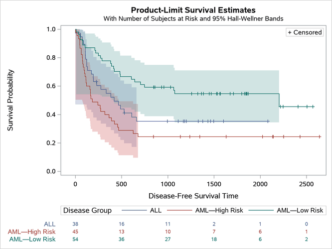
This example shows that you can save the data object and dynamic variables into SAS data sets. Then you can apply a format to the Stratum variable as you create the graph from those data sets. The advantage of this approach is that it provides full flexibility. For example, you can use it with multiple strata variables.
[24] Some dynamic variables have numeric values, and some have character values. The ODS output data set (not shown) stores the character and formatted numeric values in the variable cValue1 and the unformatted numeric values in nValue1.