The ANOVA Procedure
One-Way Layout with Means Comparisons
(View the complete code for this example.)
A one-way analysis of variance considers one treatment factor with two or more treatment levels. The goal of the analysis is to test for differences among the means of the levels and to quantify these differences. If there are two treatment levels, this analysis is equivalent to a t test comparing two group means.
The assumptions of analysis of variance (Steel and Torrie 1980) are that treatment effects are additive and experimental errors are independently random with a normal distribution that has mean zero and constant variance.
The following example studies the effect of bacteria on the nitrogen content of red clover plants. The treatment factor is bacteria strain, and it has six levels. Five of the six levels consist of different Rhizobium trifolii bacteria cultures combined with a composite of five Rhizobium meliloti strains. The sixth level is a composite of the five Rhizobium trifolii strains with the composite of the Rhizobium meliloti. Red clover plants are inoculated with the treatments, and nitrogen content is later measured in milligrams. The data are derived from an experiment by Erdman (1946) and are analyzed in Chapters 7 and 8 of Steel and Torrie (1980). The following DATA step creates the SAS data set Clover:
title1 'Nitrogen Content of Red Clover Plants';
data Clover;
   input Strain $ Nitrogen @@;
   datalines;
3DOK1  19.4 3DOK1  32.6 3DOK1  27.0 3DOK1  32.1 3DOK1  33.0
3DOK5  17.7 3DOK5  24.8 3DOK5  27.9 3DOK5  25.2 3DOK5  24.3
3DOK4  17.0 3DOK4  19.4 3DOK4   9.1 3DOK4  11.9 3DOK4  15.8
3DOK7  20.7 3DOK7  21.0 3DOK7  20.5 3DOK7  18.8 3DOK7  18.6
3DOK13 14.3 3DOK13 14.4 3DOK13 11.8 3DOK13 11.6 3DOK13 14.2
COMPOS 17.3 COMPOS 19.4 COMPOS 19.1 COMPOS 16.9 COMPOS 20.8
;
The variable Strain contains the treatment levels, and the variable Nitrogen contains the response. The following statements produce the analysis:
ods graphics on;

proc anova data = Clover;
   class Strain;
   model Nitrogen = Strain;
   means Strain / tukey;
run;
The classification variable is specified in the CLASS statement. Note that, unlike the GLM procedure, PROC ANOVA does not allow continuous variables on the right-hand side of the model. The following figures display the output produced by these statements.
Figure 1: Class Level Information
| Nitrogen Content of Red Clover Plants |
| Class Level Information | ||
|---|---|---|
| Class | Levels | Values |
| Strain | 6 | 3DOK1 3DOK13 3DOK4 3DOK5 3DOK7 COMPOS |
| Number of Observations Read | 30 |
|---|---|
| Number of Observations Used | 30 |
The "Class Level Information" table shown in Figure 1 lists the variables that appear in the CLASS statement, their levels, and the number of observations in the data set.
Figure 2 displays the ANOVA table, followed by some simple statistics and tests of effects.
Figure 2: ANOVA Table
| Nitrogen Content of Red Clover Plants |
| Source | DF | Sum of Squares | Mean Square | F Value | Pr > F |
|---|---|---|---|---|---|
| Model | 5 | 847.046667 | 169.409333 | 14.37 | <.0001 |
| Error | 24 | 282.928000 | 11.788667 | ||
| Corrected Total | 29 | 1129.974667 |
| R-Square | Coeff Var | Root MSE | Nitrogen Mean |
|---|---|---|---|
| 0.749616 | 17.26515 | 3.433463 | 19.88667 |
| Source | DF | Anova SS | Mean Square | F Value | Pr > F |
|---|---|---|---|---|---|
| Strain | 5 | 847.0466667 | 169.4093333 | 14.37 | <.0001 |
The degrees of freedom (DF) column should be used to check the analysis results. The model degrees of freedom for a one-way analysis of variance are the number of levels minus 1; in this case, 6 – 1 = 5. The Corrected Total degrees of freedom are always the total number of observations minus one; in this case 30 – 1 = 29. The sum of Model and Error degrees of freedom equals the Corrected Total.
With ODS Graphics enabled, PROC ANOVA also displays by default a plot that enables you to visualize the distribution of nitrogen content for each treatment, using a box plot of the nitrogen content values within each level of the treatment. This plot is shown in Figure 3.
Figure 3: Box Plot of Nitrogen Content for Each Treatment
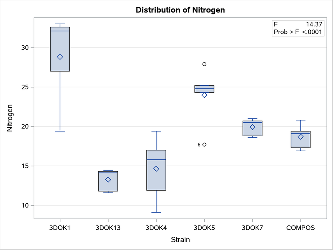
For general information about ODS Graphics, see Chapter 24, Statistical Graphics Using ODS. For specific information about the graphics available in the ANOVA procedure, see the section ODS Graphics.
The overall F test is significant  , indicating that the model as a whole accounts for a significant portion of the variability in the dependent variable. The F test for
 Strain is significant, indicating that some contrast between the means for the different strains is different from zero. Notice that the Model and Strain F tests are identical, since Strain is the only term in the model.
The significant F test for Strain suggests that there are differences among the bacterial strains, but it does not reveal any information about the nature of the differences. You can use mean comparison methods to gather further information. The MEANS statement requests comparisons of the means of the Strain levels by using Tukey’s studentized range method. Results of Tukey’s method are shown in Figure 4.
Figure 4: Tukey’s Multiple Comparisons Method
| Nitrogen Content of Red Clover Plants |
| Note: | This test controls the Type I experimentwise error rate, but it generally has a higher Type II error rate than REGWQ. |
| Alpha | 0.05 |
|---|---|
| Error Degrees of Freedom | 24 |
| Error Mean Square | 11.78867 |
| Critical Value of Studentized Range | 4.37265 |
| Minimum Significant Difference | 6.7142 |
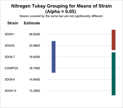
Examples of implications of the multiple comparisons results are as follows:
Strain 3DOK1 fixes significantly more nitrogen than all but 3DOK5.
While 3DOK5 is not significantly different from 3DOK1, it is also not significantly better than all the rest, though it is better than the bottom two groups.
Although the experiment has succeeded in separating the best strains from the worst, more experimentation is required in order to clearly distinguish the very best strain.