The CAUSALGRAPH Procedure

A DAG consists of three components (Elwert 2013):

Each node in the DAG represents a variable that is assumed to play a causal role in the process being studied. Each variable can have any distribution. It is not necessary for every node in the DAG to correspond to a variable that has been (or could be) measured. For example, some variables in the DAG might correspond to latent constructs that are assumed to play a causal role in the process being modeled but that cannot possibly be observed directly. By convention, error random variables (independent error terms) are not represented in a DAG (Elwert 2013) unless the error random variable is a common cause of two or more variables that the model already includes (Spirtes, Glymour, and Scheines 2001).

All edges in a DAG are directed. That is, an edge consists of an arrow that points from one node into another node. An edge is a graphical representation of a causal assumption. Specifically, an edge in a DAG represents an assumed possible direct causal effect of one variable on another (Elwert 2013). These causal effects are assumed to be deterministic (Pearl 1993), but they are fully nonparametric in the sense that each edge can have any functional form (Elwert and Winship 2014). There can be at most one edge between a pair of nodes in a DAG.

Because each edge in a DAG is given a causal interpretation, each edge is associated with a temporal ordering of a pair of nodes. For this reason, the DAG cannot contain a directed cycle. The CAUSALGRAPH procedure performs a semantic validation of every model to verify that it does not contain a directed cycle.

PROC CAUSALGRAPH allows bidirected edges to be specified. A bidirected edge is interpreted as unmeasured confounding between two variables, and thus the graph is still a DAG. For example, the edge

is interpreted as the pair of edges

where the node L represents some unmeasured variable.

Missing edges in a DAG (that is, where two nodes are not directly connected by an edge) indicate an assumption of exactly zero direct causal effect. Thus a missing edge in a DAG represents a much stronger assumption than an edge. This is the strong null hypothesis for graphical models; it is known in the econometrics literature as an exclusion restriction (Elwert 2013). Missing edges have implications for the statistical properties that are implied by a causal model. For more information about these properties, see the section Statistical Properties of Causal Models.

Together the nodes, edges, and missing edges in a DAG form a causal model that encodes researchers’ assumptions about a data generating process. Starting with these data generating assumptions, you can use a set of graphical rules that operate on the DAG to derive statements of statistical association. For more information about sources of statistical association in DAGs, see the section Sources of Association and Bias.

Two variables in a DAG are adjacent if they are directly connected by a single edge.

A path is an ordered list of variables in which no variable appears more than once and consecutive variables in the list are adjacent in the graph. The edges that connect consecutive nodes in a path can point in either direction.

A path is causal if, for every consecutive pair of variables on the path, the arrow that connects the two variables points toward the latter variable. A path that is not causal is called noncausal. A path is proper if it begins with a treatment variable and does not contain any other treatment variables (Shpitser, VanderWeele, and Robins 2010). A path can also be blocked or nonblocked. For information about blocked and nonblocked paths, see the section Statistical Properties of Causal Models.

A DAG encodes specific relationships between the variables in a causal model. It is standard practice to describe these relationships by using familial adjectives; for example, see Koller and Friedman (2009); Pearl (2009b); Elwert and Winship (2014); Van der Zander, Liśkiewicz, and Textor (2014). For an edge

P is the parent of Q and Q is the child of P. If there is a causal path from a variable S to a variable T, then T is a descendant of S and S is an ancestor of T. Thus the set of descendants of a variable S is the set of all variables that are caused (either directly or indirectly) by S. Similarly, the set of ancestors of a variable T is the set of all direct or indirect causes of T.

For a variable V on a path, V is a collider on the path if it has two arrows (one on each side) that point to it. A variable that is not a collider is a noncollider. The definition of a collider is path-specific. A variable can be a collider on one path but a noncollider on another path.

Statistical association between sets of variables can be divided into two components: a causal component and a noncausal or spurious component. If all spurious association can be removed, the causal effect is said to be identified. Identification analysis is the process of determining whether a causal effect can be identified and, if so, how to identify that effect. For more information about identification analysis, see the section Causal Effect Identification.

Spurious association is typically removed through some form of statistical adjustment or conditioning. For example, you could compute an adjustment by including a variable as a regressor in a regression model or by stratifying the analysis by levels of the variable. You can use the causal model to determine which variables must be included in an adjustment set.

A causal model that is represented by a DAG has unambiguous implications for the manner in which information can flow in the underlying data generating process. This flow of information is encapsulated by three graphical constructs that can be used to assemble every path in a DAG (Elwert 2013). The three constructs, which correspond to the three fundamental sources of association in a causal model, are as follows:

These constructs are summarized graphically in Figure 4.

Figure 4: Three Fundamental Sources of Association

In the causal structure

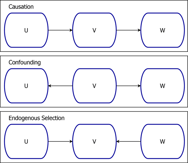
the variables U and W are associated, and this association is the result of the causal chain. If you were to condition on the mediating variable V, then this would block the flow of information such that U and W would no longer be associated.

In the confounding structure

there is no causal path that relates U and W. However, U and W are still associated. This association is induced by the confounding variable V, the common parent of U and W. If you were to condition on the common cause V, then this would block the flow of information such that U and W would no longer be associated.

In the endogenous selection structure

the variables U and W jointly determine the value of their common child V, but U and W are not associated. However, if you were to condition on the common outcome V, then this would create a flow of information such that U and W would then be associated. For examples of endogenous selection, see Elwert and Winship (2014).

Loosely speaking, if you have a treatment variable (such as U) and an outcome variable (such as W) in a causal analysis, the goal is to eliminate noncausal association between U and W and leave the causal association unchanged. Thus the three fundamental graphical constructs correspond not only to the three fundamental sources of association but also to the three fundamental sources of bias. Generally, when you have a set of treatment and outcome variables, if you control for a variable on a causal path, you block the flow of information along that causal path. This is called overcontrol bias. Similarly, if you fail to control for a confounding common cause, some of the association between the treatment and outcome variables is the result of this confounding. This is called confounding bias. Finally, if you control for a common outcome, you create association between the treatment and outcome variables that is not causal. This is called endogenous selection bias. For an accessible discussion of the three fundamental sources of association and bias, see Elwert (2013) and Elwert and Winship (2014).

There are two ways to interpret the assumptions that are encoded within a DAG:

These two interpretations are equivalent under two additional assumptions (Elwert 2013):

The local Markov property states that every variable in the DAG is statistically independent, conditional on its parents, of its set of nondescendants. In other words, the joint distribution function that is defined by the data generating process factorizes over the DAG (Koller and Friedman 2009).

The weak faithfulness property is discussed after the definition of d-separation.

A path in a DAG is said to be d-separated by a set of variables Z if either of the following conditions holds:

A path that is d-separated is said to be blocked; otherwise it is nonblocked. A set of variables X is d-separated from a set of variables Y by a set of variables Z if every path between a node in X and a node in Y is blocked.

The blocked/nonblocked terminology reflects the flow of information in a causal model. If a path is blocked, then information does not flow through that path. If the path is nonblocked, then information might flow through that path. The link between d-separation and information flow is embodied in the assumption of weak faithfulness. Weak faithfulness states that if two variables, X and Y, are not d-separated in a DAG, then the two variables are dependent in at least one distribution that factorizes over the DAG. The practical importance of faithfulness is that it does not permit the exact cancellation of the effects in a path (Elwert 2013). The use of weak faithfulness (rather than faithfulness) is consistent with the interpretation of edges as possible, rather than certain, effects (Spirtes, Glymour, and Scheines 2001; Pearl 2009b; Elwert 2013).

By interpreting a causal model as a DAG that represents the flow of association between variables, you can transform the causal assumptions that underlie a DAG into conditional independence statements. Specifically, if two variables are d-separated in a DAG by a set Z, then those two variables must be statistically independent conditional on Z. In other words, d-separation is a global Markov property. If a conditional independence statement contains only observed variables, then you can perform a statistical test by using the observed data to see whether the independence statement holds. Thus, the d-separation criterion determines the set of observationally testable implications of a causal model (Elwert 2013).

In fact, the global Markov property for DAGs (d-separation) and the local Markov property for DAGs are logically equivalent (Koller and Friedman 2009). If you have a complete list of either the local or global Markov properties, you can derive the other list by using the semigraphoid axioms (Pearl and Verma 1987; Geiger and Pearl 1988). In the CAUSALGRAPH procedure, you can use the IMAP option in the PROC CAUSALGRAPH statement to request a list of these properties.

The statistical association between a pair of variables can be divided into two components: a causal component and a noncausal or spurious component. If all spurious association can be removed, the causal effect is identified.

Identification by Adjustment

One possible approach to identification is identification by adjustment, which is the basis of causal effect identification in regression and matching (Elwert and Winship 2014). When you use identification by adjustment, you seek an adjustment set, a set of variables that, when controlled for in an analysis, blocks all the noncausal paths in a DAG without blocking any causal paths in that same DAG. The causal property of a path is inherited from the direction of the edges in a model. That is, the causal property is a property of the causal model and does not change during an analysis. However, whether a path is blocked depends not only on the structure of the DAG that represents the causal model but also on the set of variables that are included in the adjustment set. Thus, you must carefully choose an adjustment set so as to remove all confounding bias without introducing any overcontrol or endogenous selection bias.

The following criterion is necessary and sufficient for a valid adjustment set (Shpitser, VanderWeele, and Robins 2010; Perković et al. 2018). For a set of treatment variables X and a set of outcome variables Y, a set of observed variables Z is a valid adjustment set if all the following conditions are present:

• Z blocks all noncausal paths between X and Y.

• No variable in Z lies on a causal path or descends from a causal path from X to Y.

• No variable in Z is a descendant of any variable on a causal path (except possibly the variables in X).

This criterion is identical to the constructive backdoor criterion (Van der Zander, Liśkiewicz, and Textor 2014). In the CAUSALGRAPH procedure, you can specify the METHOD=ADJUSTMENT option in the PROC CAUSALGRAPH statement to list all adjustment sets that satisfy the constructive backdoor criterion.

Pearl’s backdoor criterion (Pearl 2009b) is a stronger criterion and thus can be used to produce a smaller list of adjustment sets. In PROC CAUSALGRAPH, you can specify the METHOD=BACKDOOR option to list all adjustment sets that satisfy the backdoor criterion.

Other adjustment criteria are designed to produce adjustment sets that satisfy special properties. For example, the parents-of-treatment criterion (Elwert 2013) produces adjustment sets that consist only of variables that are parents of a treatment variable. In PROC CAUSALGRAPH, you can specify the METHOD=PTREATMENT option to list all adjustment sets that satisfy the parents-of-treatment criterion. The parents-of-outcome (METHOD=POUTCOME) criterion (Elwert 2013) produces adjustment sets that consist only of variables that are parents of an outcome variable. The joint ancestor (METHOD=ANCESTOR) criterion (Elwert 2013) produces adjustment sets that consist only of variables that are ancestors of both a treatment variable and an outcome variable.

When a valid adjustment set Z has been identified, you can estimate the total causal effect of X on Y by using the stratification estimator (Shpitser, VanderWeele, and Robins 2010; Elwert 2013). For discrete data, this estimator has the form

where the do-operator is intended to emphasize the interpretation of a causal effect as the result of an action or intervention (Pearl 2009b). In the language of potential outcomes, the preceding expression describes the distribution of potential outcomes under the assumption that the potential outcome and the treatment are independent after you condition on Z. For more information about the relationship to potential outcomes, see the section Causal Graphs and Potential Outcomes.

Although the stratification estimator is fully nonparametric, it is rarely used in practice. Instead, the distribution functions in the estimator are replaced by parametric functions. This task requires considerable care and expertise. Causal effect identification is a nonparametric concept. A poorly specified parametric model can produce biased or incorrect results. For a useful summary of computational tools that you can use to estimate an average causal effect, see Schafer and Kang (2008).