The HPSPLIT Procedure
Example 68.2 Cost-Complexity Pruning with Cross Validation
(View the complete code for this example.)
In this example, data were collected to study the damage to pine forests from mountain pine beetle attacks in the Sawtooth National Recreation Area (SNRA) in Idaho (Cutler et al. 2003). (The data in this example were provided by Richard Cutler, Department of Mathematics and Statistics, Utah State University.) A classification tree is applied to classify various types of vegetation in the area based on data from satellite images. This classification can then be used to track how the pine beetle infestation is progressing through the forest. Data from 699 points in the SNRA are included in the sample.
This example creates a classification tree to predict the response variable Type, which contains the 10 vegetation classes represented in the data: Agriculture, Dirt, DougFir, Grass, GreenLP, RedTop, Road, Sagebrush, Shadow, and Water. The predictor variables include the following:
the spectral intensities on four bands of the satellite imagery:
Blue,Green,Red, andNearInfraredElevationNDVI, a function ofRedandNearInfrared"Tasseled cap transformations" of the intensities on the four bands of imagery:
SoilBrightness,Greenness,Yellowness, andNoneSuch
The first step in the analysis is to run PROC HPSPLIT to identify the best subtree model:
ods graphics on;

proc hpsplit data=sampsio.snra cvmethod=random(10) seed=123 intervalbins=500;
   class Type;
   grow gini;
   model Type = Blue Green Red NearInfrared NDVI Elevation
                SoilBrightness Greenness Yellowness NoneSuch;
   prune costcomplexity;
run;
You grow the tree by using the Gini index criterion, specified in the GROW statement, to create splits. This is a relatively small data set, so in order to use all the data to train the model, you apply cross validation with 10 folds, as specified in the CVMETHOD= option, to the cost-complexity pruning for subtree selection. An alternative would be to partition the data into training and validation sets. The SEED= option ensures that results remain the same in each run of the procedure. Different seeds can produce different trees because the cross validation fold assignments vary. When you do not specify the SEED= option, the seed is assigned based on the time.
By default, PROC HPSPLIT creates a plot of the estimated misclassification rate at each complexity parameter value in the sequence, as displayed in Figure 20.
Figure 20: Misclassification Rate as a Function of Cost-Complexity Parameter
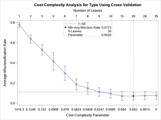
The ends of the error bars correspond to the misclassification rate plus or minus one standard error (SE) at each of the complexity pruning parameter values. A vertical reference line is drawn at the complexity parameter that has the lowest misclassification rate, and the subtree of the corresponding size for that complexity parameter is selected as the final tree. In this case, the 15-leaf tree is selected as the final tree. The horizontal reference line represents the minimum misclassification rate plus one standard error.
Often, you would apply the 1-SE rule (Breiman et al. 1984) when you are pruning via the cost-complexity method to potentially select a smaller tree that has only a slightly higher error rate than the minimum error. Selecting the smallest tree that has a misclassification rate below the horizontal reference line is in effect implementing the 1-SE rule. The subtree that has 10 leaves would be selected according to this rule, so you can run PROC HPSPLIT again as follows to override the subtree that was automatically selected in the first run:
proc hpsplit data=sampsio.snra plots=zoomedtree(node=7) seed=123 cvmodelfit
   intervalbins=500;
   class Type;
   grow gini;
   model Type = Blue Green Red NearInfrared NDVI Elevation
                SoilBrightness Greenness Yellowness NoneSuch;
   prune costcomplexity (leaves=10);
run;
This code includes specification of the LEAVES=10 option in the PRUNE statement to select this smaller subtree that performs almost equivalently to the subtree with 15 leaves from the earlier run. Specifying ZOOMEDTREE(NODE=7) in the PLOTS= option requests that the ODS graph ZoomedTreePlot displays the tree rooted at node 7 instead of at the root node. The CVMODELFIT option requests fit statistics for the final model by using cross validation as well as the cross validation confusion matrix.
Figure 21 provides an overview of the final tree that has 10 leaves as requested.
Figure 21: Diagram of 10-Leaf Tree Selected Using 1-SE Rule
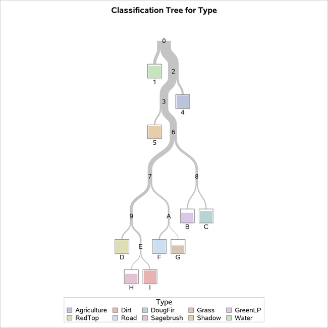
It turns out that there is exactly one leaf in the classification tree that corresponds to each of the 10 vegetation classes; this does not usually occur. The leaf color indicates the most frequently observed response among observations in that leaf, which is then the predicted response for all observations in that leaf. The height of the bars in the nodes represents the proportion of observations that have that particular response. For example, in node D, all observations have the value of RedTop for the response variable Type, whereas in node G, it appears that slightly over half of the observations have the value Grass.
Figure 22 shows more details about a portion of the final tree, including splitting variables and values.
Figure 22: Detailed Diagram of 10-Leaf Tree
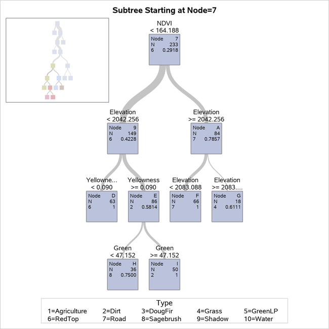
As requested, the detailed tree diagram is displayed for the portion of the tree rooted at node 7 so that you can view the splits made at the bottom of the tree. You can see that several splits are made on the variable Elevation. The vegetation type most common in node G, whose observations have an elevation of at least 2083.0880, is Grass.
Confusion matrices are displayed in Output 68.2.1.
Output 68.2.1: Confusion Matrices for SNRA Data
| Confusion Matrices | ||||||||||||
|---|---|---|---|---|---|---|---|---|---|---|---|---|
| Actual | Predicted | Error Rate |
||||||||||
| Agriculture | Dirt | DougFir | Grass | GreenLP | RedTop | Road | Sagebrush | Shadow | Water | |||
| Model Based | Agriculture | 105 | 0 | 0 | 0 | 1 | 0 | 0 | 0 | 0 | 0 | 0.0094 |
| Dirt | 0 | 50 | 0 | 0 | 1 | 0 | 0 | 0 | 0 | 2 | 0.0566 | |
| DougFir | 0 | 0 | 55 | 0 | 11 | 0 | 0 | 0 | 0 | 0 | 0.1667 | |
| Grass | 1 | 0 | 0 | 11 | 1 | 0 | 0 | 2 | 0 | 0 | 0.2667 | |
| GreenLP | 0 | 0 | 5 | 0 | 49 | 0 | 0 | 1 | 0 | 0 | 0.1091 | |
| RedTop | 0 | 0 | 0 | 5 | 0 | 63 | 0 | 0 | 0 | 0 | 0.0735 | |
| Road | 0 | 0 | 0 | 0 | 0 | 0 | 66 | 0 | 0 | 2 | 0.0294 | |
| Sagebrush | 0 | 0 | 0 | 2 | 0 | 0 | 0 | 27 | 0 | 0 | 0.0690 | |
| Shadow | 0 | 0 | 0 | 0 | 0 | 0 | 0 | 2 | 76 | 6 | 0.0952 | |
| Water | 0 | 0 | 0 | 0 | 0 | 0 | 0 | 4 | 3 | 148 | 0.0452 | |
| Cross Validation | Agriculture | 104 | 0 | 0 | 0 | 2 | 0 | 0 | 0 | 0 | 0 | 0.0189 |
| Dirt | 0 | 49 | 0 | 0 | 1 | 0 | 0 | 1 | 0 | 2 | 0.0755 | |
| DougFir | 1 | 0 | 55 | 0 | 10 | 0 | 0 | 0 | 0 | 0 | 0.1667 | |
| Grass | 2 | 0 | 0 | 11 | 0 | 0 | 0 | 2 | 0 | 0 | 0.2667 | |
| GreenLP | 0 | 0 | 16 | 0 | 37 | 0 | 0 | 1 | 1 | 0 | 0.3273 | |
| RedTop | 0 | 1 | 0 | 4 | 1 | 62 | 0 | 0 | 0 | 0 | 0.0882 | |
| Road | 0 | 0 | 0 | 0 | 0 | 2 | 64 | 0 | 0 | 2 | 0.0588 | |
| Sagebrush | 0 | 1 | 0 | 2 | 0 | 0 | 0 | 26 | 0 | 0 | 0.1034 | |
| Shadow | 0 | 0 | 0 | 0 | 0 | 2 | 0 | 2 | 74 | 6 | 0.1190 | |
| Water | 0 | 0 | 0 | 0 | 0 | 3 | 0 | 1 | 3 | 148 | 0.0452 | |
This table contains two matrices—one for the training data that uses the final tree and one that uses the cross validation folds—requested by the CVMODELFIT option in the PROC HPSPLIT statement. The values on the diagonal of each confusion matrix are the number of observations that are correctly classified for each of the 10 vegetation types. For the model-based matrix, you can see that the only nonzero value in the RedTop column is in the RedTop row. This is consistent with what is shown in Figure 21, where the bar in node D with a predicted response of RedTop is the full height of the box representing the leaf, indicating that all observations on that leaf are correctly classified. You can also see from the matrix that the DougFir and GreenLP vegetation types are hard to distinguish; 11 of the 66 observations that have an actual response of DougFir are incorrectly assigned the response of GreenLP, corresponding to the 0.1667 error rate reported for DougFir.
Fit statistics are shown in Output 68.2.2.
Output 68.2.2: Fit Statistics for SNRA Data
| Fit Statistics for Selected Tree | ||||||
|---|---|---|---|---|---|---|
| N Leaves |
ASE | Mis- class |
Entropy | Gini | RSS | |
| Model Based | 10 | 0.0120 | 0.0701 | 0.3597 | 0.1197 | 83.6514 |
| Cross Validation | 10 | 0.0166 | 0.0974 | |||
You can see from this table that the subtree with 10 leaves fits the training data very accurately, with 93% of the observations classified correctly. Because no validation data are present in this analysis, you get a better indication of how well the model fits and will generalize to new data by looking at the cross validation statistics, also requested by the CVMODELFIT option, that are included in the table. The misclassification rate that is averaged across the 10 folds is higher than the training misclassification rate for the final tree, suggesting that this model is slightly overfitting the training data.