Introduction to Clustering Procedures
Elongated Multinormal Clusters
In this example, the data are sampled from two highly elongated multinormal distributions with equal covariance matrices. The following SAS statements produce Figure 18:
data elongate;
   keep x y;
   ma=8; mb=0; link generate;
   ma=6; mb=8; link generate;
   stop;
generate:
   do i=1 to 50;
      a=rannor(7)*6+ma;
      b=rannor(7)+mb;
      x=a-b;
      y=a+b;
      output;
   end;
   return;
run;
proc fastclus data=elongate out=out maxc=2 noprint;
run;
proc sgplot noautolegend;
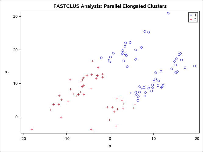
title 'FASTCLUS Analysis: Parallel Elongated Clusters';
scatter y=y x=x / group=cluster;
keylegend / location=inside position=topright sortorder=ascending
across=1 noopaque title='';
run;
Notice that PROC FASTCLUS found two clusters, as requested by the MAXC= option. However, it attempted to form spherical clusters, which are obviously inappropriate for these data.
Figure 18: Parallel Elongated Clusters: PROC FASTCLUS
The following SAS statements produce Figure 19:
proc cluster data=elongate outtree=tree method=average noprint;
run;

proc tree noprint out=out n=2 dock=5;
   copy x y;
run;

proc sgplot noautolegend;
   title 'Average Linkage Cluster Analysis: '
         'Parallel Elongated Clusters';
   scatter y=y x=x / group=cluster;
   keylegend / location=inside position=topright sortorder=ascending
               across=1 noopaque title='';
run;
Figure 19: Parallel Elongated Clusters: PROC CLUSTER METHOD=AVERAGE

The following SAS statements produce Figure 20:
proc cluster data=elongate outtree=tree method=twostage k=10 noprint;
run;

proc tree noprint out=out n=2;
   copy x y;
run;

proc sgplot noautolegend;
   title 'Two-Stage Density Linkage Cluster Analysis: '
         'Parallel Elongated Clusters';
   scatter y=y x=x / group=cluster;
   keylegend / location=inside position=topright sortorder=ascending
               across=1 noopaque title='';
run;
Figure 20: Parallel Elongated Clusters: PROC CLUSTER METHOD=TWOSTAGE
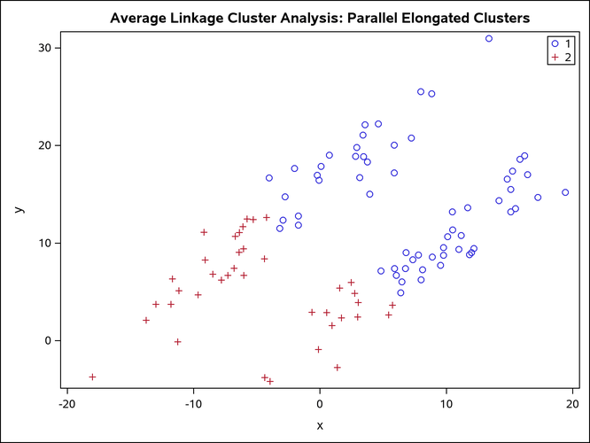
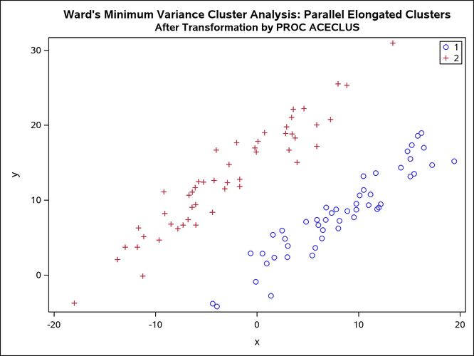
PROC FASTCLUS and average linkage fail miserably. Ward’s method and the centroid method (not shown) produce almost the same results. Two-stage density linkage, however, recovers the correct clusters. Single linkage (not shown) finds the same clusters as two-stage density linkage except for some outliers.
In this example, the population clusters have equal covariance matrices. If the within-cluster covariances are known, the data can be transformed to make the clusters spherical so that any of the clustering methods can find the correct clusters. But when you are doing a cluster analysis, you do not know what the true clusters are, so you cannot calculate the within-cluster covariance matrix. Nevertheless, it is sometimes possible to estimate the within-cluster covariance matrix without knowing the cluster membership or even the number of clusters, using an approach invented by Art, Gnanadesikan, and Kettenring (1982). A method for obtaining such an estimate is available in the ACECLUS procedure.
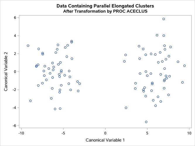
In the following analysis, PROC ACECLUS transforms the variables X and Y into the canonical variables Can1 and Can2. The latter are plotted and then used in a cluster analysis by Ward’s method. The clusters are then plotted with the original variables X and Y.
The following SAS statements produce Figure 21 and Figure 22:
proc aceclus data=elongate out=ace p=.1;
   var x y;
   title 'ACECLUS Analysis: Parallel Elongated Clusters';
run;

proc sgplot noautolegend;
   title 'Data Containing Parallel Elongated Clusters';
   title2 'After Transformation by PROC ACECLUS';
   scatter y=can2 x=can1;
   xaxis label='Canonical Variable 1';
   yaxis label='Canonical Variable 2';
run;
Figure 21: Parallel Elongated Clusters: PROC ACECLUS
| ACECLUS Analysis: Parallel Elongated Clusters |
| Observations | 100 | Proportion | 0.1000 |
|---|---|---|---|
| Variables | 2 | Converge | 0.00100 |
| Means and Standard Deviations | ||
|---|---|---|
| Variable | Mean | Standard Deviation |
| x | 2.6406 | 8.3494 |
| y | 10.6488 | 6.8420 |
| COV: Total Sample Covariances | ||
|---|---|---|
| x | y | |
| x | 69.71314819 | 24.24268934 |
| y | 24.24268934 | 46.81324861 |
| Initial Within-Cluster Covariance Estimate = Full Covariance Matrix |
| Threshold = | 0.328478 |
|---|
| Iteration History | ||||
|---|---|---|---|---|
| Iteration | RMS Distance |
Distance Cutoff |
Pairs Within Cutoff |
Convergence Measure |
| 1 | 2.000 | 0.657 | 672.0 | 0.673685 |
| 2 | 9.382 | 3.082 | 716.0 | 0.006963 |
| 3 | 9.339 | 3.068 | 760.0 | 0.008362 |
| 4 | 9.437 | 3.100 | 824.0 | 0.009656 |
| 5 | 9.359 | 3.074 | 889.0 | 0.010269 |
| 6 | 9.267 | 3.044 | 955.0 | 0.011276 |
| 7 | 9.208 | 3.025 | 999.0 | 0.009230 |
| 8 | 9.230 | 3.032 | 1052.0 | 0.011394 |
| 9 | 9.226 | 3.030 | 1091.0 | 0.007924 |
| 10 | 9.173 | 3.013 | 1121.0 | 0.007993 |
| WARNING: Iteration limit exceeded. |
| ACE: Approximate Covariance Estimate Within Clusters |
||
|---|---|---|
| x | y | |
| x | 9.299329632 | 8.215362614 |
| y | 8.215362614 | 8.937753936 |
| Eigenvalues of Inv(ACE)*(COV-ACE) | ||||
|---|---|---|---|---|
| Eigenvalue | Difference | Proportion | Cumulative | |
| 1 | 36.7091 | 33.1672 | 0.9120 | 0.9120 |
| 2 | 3.5420 | 0.0880 | 1.0000 | |
| Eigenvectors (Raw Canonical Coefficients) |
||
|---|---|---|
| Can1 | Can2 | |
| x | -.748392 | 0.109547 |
| y | 0.736349 | 0.230272 |
| Standardized Canonical Coefficients |
||
|---|---|---|
| Can1 | Can2 | |
| x | -6.24866 | 0.91466 |
| y | 5.03812 | 1.57553 |
Figure 22: Parallel Elongated Clusters after Transformation by PROC ACECLUS
The following SAS statements produce Figure 23:
proc cluster data=ace outtree=tree method=ward noprint;
   var can1 can2;
   copy x y;
run;

proc tree noprint out=out n=2;
   copy x y;
run;

proc sgplot noautolegend;
   title 'Ward''s Minimum Variance Cluster Analysis: '
         'Parallel Elongated Clusters';
   title2 'After Transformation by PROC ACECLUS';
   scatter y=y x=x / group=cluster;
   keylegend / location=inside position=topright sortorder=ascending
               across=1 noopaque title='';
run;
Figure 23: Transformed Data Containing Parallel Elongated Clusters: PROC CLUSTER METHOD=WARD