The MIXED Procedure
ODS Graphics
Statistical procedures use ODS Graphics to create graphs as part of their output. ODS Graphics is described in detail in Chapter 24, Statistical Graphics Using ODS.
Before you create graphs, ODS Graphics must be enabled (for example, by specifying the ODS GRAPHICS ON statement). For more information about enabling and disabling ODS Graphics, see the section Enabling and Disabling ODS Graphics in Chapter 24, Statistical Graphics Using ODS.
The overall appearance of graphs is controlled by ODS styles. Styles and other aspects of using ODS Graphics are discussed in the section A Primer on ODS Statistical Graphics in Chapter 24, Statistical Graphics Using ODS.
Some graphs are produced by default; other graphs are produced by using statements and options.
ODS Graph Names
You can reference every graph produced through ODS Graphics with a name. The names of the graphs that PROC MIXED generates are listed in Table 28, along with the required statements and options.
Table 28: Graphs Produced by PROC MIXED
| ODS Graph Name | Plot Description | Statement or Option |
|---|---|---|
| Boxplot | Box plots | PLOTS=BOXPLOT |
| CovRatioPlot | CovRatio statistics for fixed effects or covariance parameters | PLOTS=INFLUENCESTATPANEL(UNPACK) and MODEL / INFLUENCE |
| CooksDPlot | Cook’s D for fixed effects or covariance parameters | PLOTS=INFLUENCESTATPANEL(UNPACK) and MODEL / INFLUENCE |
| DistancePlot | Likelihood or restricted likelihood distance | MODEL / INFLUENCE |
| InfluenceEstPlot | Panel of deletion estimates | MODEL / INFLUENCE(EST) or PLOTS=INFLUENCEESTPLOT and MODEL / INFLUENCE |
| InfluenceEstPlot | Parameter estimates after removing observation or sets of observations | PLOTS=INFLUENCEESTPLOT(UNPACK) and MODEL / INFLUENCE |
| InfluenceStatPanel | Panel of influence statistics | MODEL / INFLUENCE |
| PearsonBoxPlot | Box plot of Pearson residuals | PLOTS=PEARSONPANEL(UNPACK BOX) |
| PearsonByPredicted | Pearson residuals vs. predicted | PLOTS=PEARSONPANEL(UNPACK) |
| PearsonHistogram | Histogram of Pearson residuals | PLOTS=PEARSONPANEL(UNPACK) |
| PearsonPanel | Panel of Pearson residuals | MODEL / RESIDUAL |
| PearsonQQplot | Q-Q plot of Pearson residuals | PLOTS=PEARSONPANEL(UNPACK) |
| PressPlot | Plot of PRESS residuals or PRESS statistic | PLOTS=PRESS and MODEL / INFLUENCE |
| ResidualBoxplot | Box plot of (raw) residuals | PLOTS=RESIDUALPANEL(UNPACK BOX) |
| ResidualByPredicted | Residuals vs. predicted | PLOTS=RESIDUALPANEL(UNPACK) |
| ResidualHistogram | Histogram of raw residuals | PLOTS=RESIDUALPANEL(UNPACK) |
| ResidualPanel | Panel of (raw) residuals | MODEL / RESIDUAL |
| ResidualQQplot | Q-Q plot of raw residuals | PLOTS=RESIDUALPANEL(UNPACK) |
| ScaledBoxplot | Box plot of scaled residuals | PLOTS=VCIRYPANEL(UNPACK BOX) |
| ScaledByPredicted | Scaled residuals vs. predicted | PLOTS=VCIRYPANEL(UNPACK) |
| ScaledHistogram | Histogram of scaled residuals | PLOTS=VCIRYPANEL(UNPACK) |
| ScaledQQplot | Q-Q plot of scaled residuals | PLOTS=VCIRYPANEL(UNPACK) |
| StudentBoxplot | Box plot of studentized residuals | PLOTS=STUDENTPANEL(UNPACK BOX) |
| StudentByPredicted | Studentized residuals vs. predicted | PLOTS=STUDENTPANEL(UNPACK) |
| StudentHistogram | Histogram of studentized residuals | PLOTS=STUDENTPANEL(UNPACK) |
| StudentPanel | Panel of studentized residuals | MODEL / RESIDUAL |
| StudentQQplot | Q-Q plot of studentized residuals | PLOTS=STUDENTPANEL(UNPACK) |
| VCIRYPanel | Panel of scaled residuals | MODEL / VCIRY |
When ODS Graphics is enabled, the LSMESTIMATE and SLICE statements can produce plots that are associated with their analyses. For information about these plots, see the sections LSMESTIMATE Statement and SLICE Statement in Chapter 20, Shared Concepts and Topics.
Residual Plots
The MIXED procedure can generate panels of residual diagnostics. Each panel consists of a plot of residuals versus predicted values, a histogram with normal density overlaid, a Q-Q plot, and summary residual and fit statistics (Figure 15). The plots are produced even if the OUTP= and OUTPM= options in the MODEL statement are not specified. Residual panels can be generated for marginal and conditional raw, studentized, and Pearson residuals as well as for scaled residuals (see the section Residual Diagnostics).
Recall the example in the section Getting Started: MIXED Procedure. The following statements generate several  panels of residual graphs:
ods graphics on;
proc mixed data=heights plots=studentpanel(marginal conditional);
   class Family Gender;
   model Height = Gender / residual;
   random Family Family*Gender;
run;
ods graphics off;
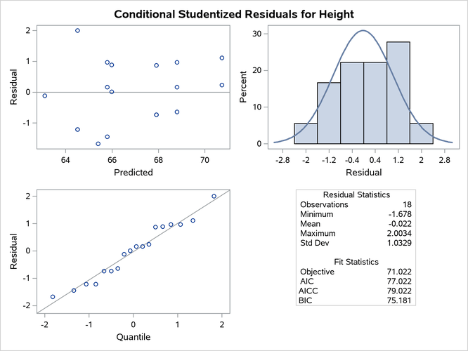
The graphs are created when ODS Graphics is enabled. The panel of the studentized marginal residuals is shown in Figure 15, and the panel of the studentized conditional residuals is shown in Figure 16.
Figure 15: Panel of the Studentized (Marginal) Residuals
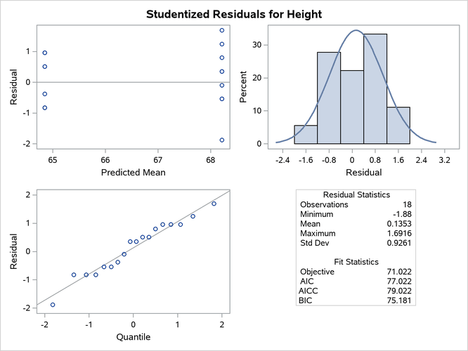
Since the fixed-effects part of the model comprises only an intercept and the gender effect, the marginal mean takes on only two values, one for each gender. The "Residual Statistics" inset in the lower-right corner provides descriptive statistics for the set of residuals that is displayed. Note that residuals in a mixed model do not necessarily sum to zero, even if the model contains an intercept.
Figure 16: Panel of the Conditional Studentized Residuals
Influence Plots
The graphical features of the MIXED procedure enable you to generate plots of influence diagnostics and of deletion estimates. The type and number of plots produced depend on your modifiers of the INFLUENCE option in the MODEL statement and on the PLOTS= option in the PROC MIXED statement. Plots related to covariance parameters are produced only when diagnostics are computed by iterative methods (ITER=). The estimates of the fixed effects—and covariance parameters when updates are iterative—are plotted when you specify the ESTIMATES modifier or when you request PLOTS=INFLUENCEESTPLOT.
Two basic types of influence panels are shown in Figure 17 and Figure 18. The diagnostics panel shows Cook’s D and CovRatio statistics for the fixed effects and the covariance parameters. For the SAS statements that produce these influence panels, see Example 84.8. In this example, the impact of subjects (Person) on the analysis is assessed. The Cook’s D statistic measures a subject’s impact on the estimates, and the CovRatio statistic measures a subject’s impact on the precision of the estimates. Separate statistics are computed for the fixed effects and the covariance parameters. The CovRatio statistic has a threshold of 1.0. Values larger than 1.0 indicate that precision of the estimates is lost by exclusion of the observations in question. Values smaller than 1.0 indicate that precision is gained by exclusion of the observations from the analysis. For example, it is evident from Figure 17 that person 20 has considerable impact on the covariance parameter estimates and moderate influence on the fixed-effects estimates. Furthermore, exclusion of this subject from the analysis increases the precision of the covariance parameters, whereas the effect on the precision of the fixed effects is minor.
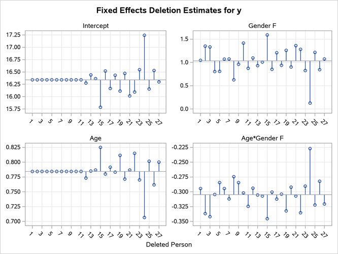
Figure 18 shows another type of influence plot, a panel of the deletion estimates. Each plot within the panel corresponds to one of the model parameters. A reference line is drawn at the estimate based on the full data.
Figure 17: Influence Diagnostics
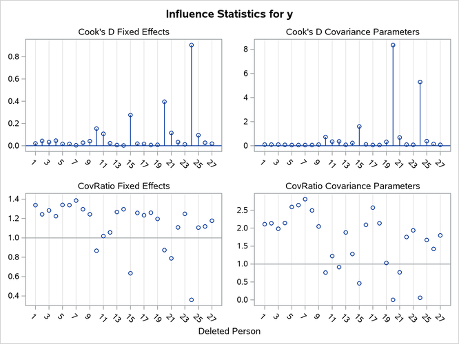
Figure 18: Deletion Estimates