The MIXED Procedure
Example 84.3 Plotting the Likelihood
(View the complete code for this example.)
The data for this example are from Hemmerle and Hartley (1973) and are also used for an example in the VARCOMP procedure. The response variable consists of measurements from an oven experiment, and the model contains a fixed effect A and random effects B and A*B.
The SAS statements are as follows:
data hh;
   input a b y @@;
   datalines;
1 1 237   1 1 254    1 1 246
1 2 178   1 2 179
2 1 208   2 1 178    2 1 187
2 2 146   2 2 145    2 2 141
3 1 186   3 1 183
3 2 142   3 2 125    3 2 136
;
ods output ParmSearch=parms;
proc mixed data=hh asycov mmeq mmeqsol covtest;
   class a b;
   model y = a / outp=predicted;
   random b a*b;
   lsmeans a;
   parms (17 to 20 by .1) (.3 to .4 by .005) (1.0);
run;
proc print data=predicted;
run;
The ASYCOV option in the PROC MIXED statement requests the asymptotic variance matrix of the covariance parameter estimates. This matrix is the observed inverse Fisher information matrix, which equals  , where
  is the Hessian matrix of the objective function evaluated at the final covariance parameter estimates. The MMEQ and MMEQSOL options in the PROC MIXED statement request that the mixed model equations and their solution be displayed.
The OUTP= option in the MODEL statement produces the data set predicted, containing the predicted values. Least squares means (LSMEANS) are requested for A. The PARMS and ODS statements are used to construct a data set containing the likelihood surface.
The results from this analysis are shown in Figure 52–Output 84.3.2.
The "Model Information" table in Figure 52 lists details about this variance components model.
Figure 52: Model Information
| Model Information | |
|---|---|
| Data Set | WORK.HH |
| Dependent Variable | y |
| Covariance Structure | Variance Components |
| Estimation Method | REML |
| Residual Variance Method | Profile |
| Fixed Effects SE Method | Model-Based |
| Degrees of Freedom Method | Containment |
The "Class Level Information" table in Figure 53 lists the levels for A and B.
Figure 53: Class Level Information
| Class Level Information | ||
|---|---|---|
| Class | Levels | Values |
| a | 3 | 1 2 3 |
| b | 2 | 1 2 |
The "Dimensions" table in Figure 54 reveals that  is
is  and
and  is
is  . Since there are no SUBJECT= effects, PROC MIXED considers the data to be effectively from one subject with 16 observations.
Figure 54: Model Dimensions and Number of Observations
| Dimensions | |
|---|---|
| Covariance Parameters | 3 |
| Columns in X | 4 |
| Columns in Z | 8 |
| Subjects | 1 |
| Max Obs per Subject | 16 |
| Number of Observations | |
|---|---|
| Number of Observations Read | 16 |
| Number of Observations Used | 16 |
| Number of Observations Not Used | 0 |
Only a portion of the "Parameter Search" table is shown in Output 84.3.1 because the full listing has 651 rows.
Output 84.3.1: Selected Results of Parameter Search
| The Mixed Procedure |
| CovP1 | CovP2 | CovP3 | Variance | Res Log Like | -2 Res Log Like |
|---|---|---|---|---|---|
| 17.0000 | 0.3000 | 1.0000 | 80.1400 | -52.4699 | 104.9399 |
| 17.0000 | 0.3050 | 1.0000 | 80.0466 | -52.4697 | 104.9393 |
| 17.0000 | 0.3100 | 1.0000 | 79.9545 | -52.4694 | 104.9388 |
| 17.0000 | 0.3150 | 1.0000 | 79.8637 | -52.4692 | 104.9384 |
| 17.0000 | 0.3200 | 1.0000 | 79.7742 | -52.4691 | 104.9381 |
| 17.0000 | 0.3250 | 1.0000 | 79.6859 | -52.4690 | 104.9379 |
| 17.0000 | 0.3300 | 1.0000 | 79.5988 | -52.4689 | 104.9378 |
| 17.0000 | 0.3350 | 1.0000 | 79.5129 | -52.4689 | 104.9377 |
| 17.0000 | 0.3400 | 1.0000 | 79.4282 | -52.4689 | 104.9377 |
| 17.0000 | 0.3450 | 1.0000 | 79.3447 | -52.4689 | 104.9378 |
| . | . | . | . | . | . |
| . | . | . | . | . | . |
| . | . | . | . | . | . |
| 20.0000 | 0.3550 | 1.0000 | 78.2003 | -52.4683 | 104.9366 |
| 20.0000 | 0.3600 | 1.0000 | 78.1201 | -52.4684 | 104.9368 |
| 20.0000 | 0.3650 | 1.0000 | 78.0409 | -52.4685 | 104.9370 |
| 20.0000 | 0.3700 | 1.0000 | 77.9628 | -52.4687 | 104.9373 |
| 20.0000 | 0.3750 | 1.0000 | 77.8857 | -52.4689 | 104.9377 |
| 20.0000 | 0.3800 | 1.0000 | 77.8096 | -52.4691 | 104.9382 |
| 20.0000 | 0.3850 | 1.0000 | 77.7345 | -52.4693 | 104.9387 |
| 20.0000 | 0.3900 | 1.0000 | 77.6603 | -52.4696 | 104.9392 |
| 20.0000 | 0.3950 | 1.0000 | 77.5871 | -52.4699 | 104.9399 |
| 20.0000 | 0.4000 | 1.0000 | 77.5148 | -52.4703 | 104.9406 |
As Figure 55 shows, convergence occurs quickly because PROC MIXED starts from the best value from the grid search.
Figure 55: Iteration History and Convergence Status
| Iteration History | |||
|---|---|---|---|
| Iteration | Evaluations | -2 Res Log Like | Criterion |
| 1 | 2 | 104.93416367 | 0.00000000 |
| Convergence criteria met. |
The "Covariance Parameter Estimates" table in Figure 56 lists the variance components estimates. Note that B is much more variable than A*B.
Figure 56: Estimated Covariance Parameters
| Covariance Parameter Estimates | ||||
|---|---|---|---|---|
| Cov Parm | Estimate | Standard Error |
Z Value | Pr > Z |
| b | 1464.36 | 2098.01 | 0.70 | 0.2426 |
| a*b | 26.9581 | 59.6570 | 0.45 | 0.3257 |
| Residual | 78.8426 | 35.3512 | 2.23 | 0.0129 |
The asymptotic covariance matrix in Figure 57 also reflects the large variability of B relative to A*B.
Figure 57: Asymptotic Covariance Matrix of Covariance Parameters
| Asymptotic Covariance Matrix of Estimates | ||||
|---|---|---|---|---|
| Row | Cov Parm | CovP1 | CovP2 | CovP3 |
| 1 | b | 4401640 | 1.2831 | -273.32 |
| 2 | a*b | 1.2831 | 3558.96 | -502.84 |
| 3 | Residual | -273.32 | -502.84 | 1249.71 |
As Figure 58 shows, the PARMS likelihood ratio test (LRT) compares the best model from the grid search with the final fitted model. Since these models are nearly the same, the LRT is not significant.
Figure 58: Fit Statistics and Likelihood Ratio Test
| Fit Statistics | |
|---|---|
| -2 Res Log Likelihood | 104.9 |
| AIC (Smaller is Better) | 110.9 |
| AICC (Smaller is Better) | 113.6 |
| BIC (Smaller is Better) | 107.0 |
| PARMS Model Likelihood Ratio Test | ||
|---|---|---|
| DF | Chi-Square | Pr > ChiSq |
| 2 | 0.00 | 1.0000 |
The mixed model equations are analogous to the normal equations in the standard linear model. As Figure 59 shows, for this example, rows 1–4 correspond to the fixed effects, rows 5–12 correspond to the random effects, and Col13 corresponds to the dependent variable.
Figure 59: Mixed Model Equations
| Mixed Model Equations | ||||||||||||||||
|---|---|---|---|---|---|---|---|---|---|---|---|---|---|---|---|---|
| Row | Effect | a | b | Col1 | Col2 | Col3 | Col4 | Col5 | Col6 | Col7 | Col8 | Col9 | Col10 | Col11 | Col12 | Col13 |
| 1 | Intercept | 0.2029 | 0.06342 | 0.07610 | 0.06342 | 0.1015 | 0.1015 | 0.03805 | 0.02537 | 0.03805 | 0.03805 | 0.02537 | 0.03805 | 36.4143 | ||
| 2 | a | 1 | 0.06342 | 0.06342 | 0.03805 | 0.02537 | 0.03805 | 0.02537 | 13.8757 | |||||||
| 3 | a | 2 | 0.07610 | 0.07610 | 0.03805 | 0.03805 | 0.03805 | 0.03805 | 12.7469 | |||||||
| 4 | a | 3 | 0.06342 | 0.06342 | 0.02537 | 0.03805 | 0.02537 | 0.03805 | 9.7917 | |||||||
| 5 | b | 1 | 0.1015 | 0.03805 | 0.03805 | 0.02537 | 0.1022 | 0.03805 | 0.03805 | 0.02537 | 21.2956 | |||||
| 6 | b | 2 | 0.1015 | 0.02537 | 0.03805 | 0.03805 | 0.1022 | 0.02537 | 0.03805 | 0.03805 | 15.1187 | |||||
| 7 | a*b | 1 | 1 | 0.03805 | 0.03805 | 0.03805 | 0.07515 | 9.3477 | ||||||||
| 8 | a*b | 1 | 2 | 0.02537 | 0.02537 | 0.02537 | 0.06246 | 4.5280 | ||||||||
| 9 | a*b | 2 | 1 | 0.03805 | 0.03805 | 0.03805 | 0.07515 | 7.2676 | ||||||||
| 10 | a*b | 2 | 2 | 0.03805 | 0.03805 | 0.03805 | 0.07515 | 5.4793 | ||||||||
| 11 | a*b | 3 | 1 | 0.02537 | 0.02537 | 0.02537 | 0.06246 | 4.6802 | ||||||||
| 12 | a*b | 3 | 2 | 0.03805 | 0.03805 | 0.03805 | 0.07515 | 5.1115 | ||||||||
The solution matrix in Figure 60 results from sweeping all but the last row of the mixed model equations matrix. The final column contains a solution vector for the fixed and random effects. The first four rows correspond to fixed effects and the last eight correspond to random effects.
Figure 60: Solutions of the Mixed Model Equations
| Mixed Model Equations Solution | ||||||||||||||||
|---|---|---|---|---|---|---|---|---|---|---|---|---|---|---|---|---|
| Row | Effect | a | b | Col1 | Col2 | Col3 | Col4 | Col5 | Col6 | Col7 | Col8 | Col9 | Col10 | Col11 | Col12 | Col13 |
| 1 | Intercept | 761.84 | -29.7718 | -29.6578 | -731.14 | -733.22 | -0.4680 | 0.4680 | -0.5257 | 0.5257 | -12.4663 | -14.4918 | 159.61 | |||
| 2 | a | 1 | -29.7718 | 59.5436 | 29.7718 | -2.0764 | 2.0764 | -14.0239 | -12.9342 | 1.0514 | -1.0514 | 12.9342 | 14.0239 | 53.2049 | ||
| 3 | a | 2 | -29.6578 | 29.7718 | 56.2773 | -1.0382 | 1.0382 | 0.4680 | -0.4680 | -12.9534 | -14.0048 | 12.4663 | 14.4918 | 7.8856 | ||
| 4 | a | 3 | ||||||||||||||
| 5 | b | 1 | -731.14 | -2.0764 | -1.0382 | 741.63 | 722.73 | -4.2598 | 4.2598 | -4.7855 | 4.7855 | -4.2598 | 4.2598 | 26.8837 | ||
| 6 | b | 2 | -733.22 | 2.0764 | 1.0382 | 722.73 | 741.63 | 4.2598 | -4.2598 | 4.7855 | -4.7855 | 4.2598 | -4.2598 | -26.8837 | ||
| 7 | a*b | 1 | 1 | -0.4680 | -14.0239 | 0.4680 | -4.2598 | 4.2598 | 22.8027 | 4.1555 | 2.1570 | -2.1570 | 1.9200 | -1.9200 | 3.0198 | |
| 8 | a*b | 1 | 2 | 0.4680 | -12.9342 | -0.4680 | 4.2598 | -4.2598 | 4.1555 | 22.8027 | -2.1570 | 2.1570 | -1.9200 | 1.9200 | -3.0198 | |
| 9 | a*b | 2 | 1 | -0.5257 | 1.0514 | -12.9534 | -4.7855 | 4.7855 | 2.1570 | -2.1570 | 22.5560 | 4.4021 | 2.1570 | -2.1570 | -1.7134 | |
| 10 | a*b | 2 | 2 | 0.5257 | -1.0514 | -14.0048 | 4.7855 | -4.7855 | -2.1570 | 2.1570 | 4.4021 | 22.5560 | -2.1570 | 2.1570 | 1.7134 | |
| 11 | a*b | 3 | 1 | -12.4663 | 12.9342 | 12.4663 | -4.2598 | 4.2598 | 1.9200 | -1.9200 | 2.1570 | -2.1570 | 22.8027 | 4.1555 | -0.8115 | |
| 12 | a*b | 3 | 2 | -14.4918 | 14.0239 | 14.4918 | 4.2598 | -4.2598 | -1.9200 | 1.9200 | -2.1570 | 2.1570 | 4.1555 | 22.8027 | 0.8115 | |
The A factor is significant at the 5% level (Figure 61).
Figure 61: Tests of Fixed Effects
| Type 3 Tests of Fixed Effects | ||||
|---|---|---|---|---|
| Effect | Num DF | Den DF | F Value | Pr > F |
| a | 2 | 2 | 28.00 | 0.0345 |
Figure 62 shows that the significance of A appears to be from the difference between its first level and its other two levels.
Figure 62: Least Squares Means for A Effect
| Least Squares Means | ||||||
|---|---|---|---|---|---|---|
| Effect | a | Estimate | Standard Error |
DF | t Value | Pr > |t| |
| a | 1 | 212.82 | 27.6014 | 2 | 7.71 | 0.0164 |
| a | 2 | 167.50 | 27.5463 | 2 | 6.08 | 0.0260 |
| a | 3 | 159.61 | 27.6014 | 2 | 5.78 | 0.0286 |
Output 84.3.2 lists the predicted values from the model. These values are the sum of the fixed-effects estimates and the empirical best linear unbiased predictors (EBLUPs) of the random effects.
Output 84.3.2: Predicted Values
| Obs | a | b | y | Pred | StdErrPred | DF | Alpha | Lower | Upper | Resid |
|---|---|---|---|---|---|---|---|---|---|---|
| 1 | 1 | 1 | 237 | 242.723 | 4.72563 | 10 | 0.05 | 232.193 | 253.252 | -5.7228 |
| 2 | 1 | 1 | 254 | 242.723 | 4.72563 | 10 | 0.05 | 232.193 | 253.252 | 11.2772 |
| 3 | 1 | 1 | 246 | 242.723 | 4.72563 | 10 | 0.05 | 232.193 | 253.252 | 3.2772 |
| 4 | 1 | 2 | 178 | 182.916 | 5.52589 | 10 | 0.05 | 170.603 | 195.228 | -4.9159 |
| 5 | 1 | 2 | 179 | 182.916 | 5.52589 | 10 | 0.05 | 170.603 | 195.228 | -3.9159 |
| 6 | 2 | 1 | 208 | 192.670 | 4.70076 | 10 | 0.05 | 182.196 | 203.144 | 15.3297 |
| 7 | 2 | 1 | 178 | 192.670 | 4.70076 | 10 | 0.05 | 182.196 | 203.144 | -14.6703 |
| 8 | 2 | 1 | 187 | 192.670 | 4.70076 | 10 | 0.05 | 182.196 | 203.144 | -5.6703 |
| 9 | 2 | 2 | 146 | 142.330 | 4.70076 | 10 | 0.05 | 131.856 | 152.804 | 3.6703 |
| 10 | 2 | 2 | 145 | 142.330 | 4.70076 | 10 | 0.05 | 131.856 | 152.804 | 2.6703 |
| 11 | 2 | 2 | 141 | 142.330 | 4.70076 | 10 | 0.05 | 131.856 | 152.804 | -1.3297 |
| 12 | 3 | 1 | 186 | 185.687 | 5.52589 | 10 | 0.05 | 173.374 | 197.999 | 0.3134 |
| 13 | 3 | 1 | 183 | 185.687 | 5.52589 | 10 | 0.05 | 173.374 | 197.999 | -2.6866 |
| 14 | 3 | 2 | 142 | 133.542 | 4.72563 | 10 | 0.05 | 123.013 | 144.072 | 8.4578 |
| 15 | 3 | 2 | 125 | 133.542 | 4.72563 | 10 | 0.05 | 123.013 | 144.072 | -8.5422 |
| 16 | 3 | 2 | 136 | 133.542 | 4.72563 | 10 | 0.05 | 123.013 | 144.072 | 2.4578 |
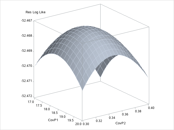
To plot the likelihood surface by using ODS Graphics, use the following statements:
proc template;
   define statgraph surface;
      begingraph;
         layout overlay3d;
            surfaceplotparm x=CovP1 y=CovP2 z=ResLogLike;
         endlayout;
      endgraph;
   end;
run;
proc sgrender data=parms template=surface;
run;
The results from this plot are shown in Output 84.3.3. The peak of the surface is the REML estimates for the B and A*B variance components.
Output 84.3.3: Plot of Likelihood Surface