Statistical Graphics Using ODS

This example is taken from the section Getting Started: KDE Procedure in Chapter 73, The KDE Procedure. Here, in addition to the ODS GRAPHICS statement, procedure options are used to request plots. The following statements simulate 1,000 observations from a bivariate normal density that has means (0,0), variances (10,10), and covariance 9:

data bivnormal;
   do i = 1 to 1000;
      z1 = rannor(104);
      z2 = rannor(104);
      z3 = rannor(104);
      x  = 3*z1+z2;
      y  = 3*z1+z3;
      output;
   end;
run;

The following statements request a bivariate kernel density estimate for the variables x and y:

proc kde data=bivnormal;
   bivar x y / plots=contour surface;
run;

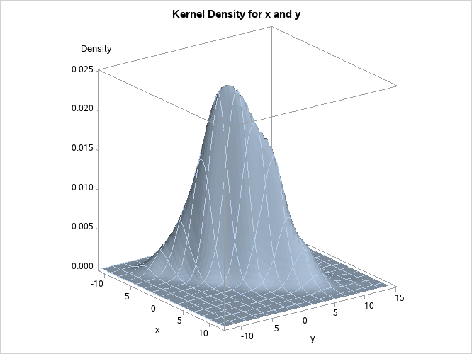
The PLOTS= option requests a contour plot and a surface plot of the estimate (displayed in Figure 5 and Figure 6, respectively). For more information about the graphs available in PROC KDE, see the section ODS Graphics in Chapter 73, The KDE Procedure.

Figure 5: Contour Plot of Estimated Density

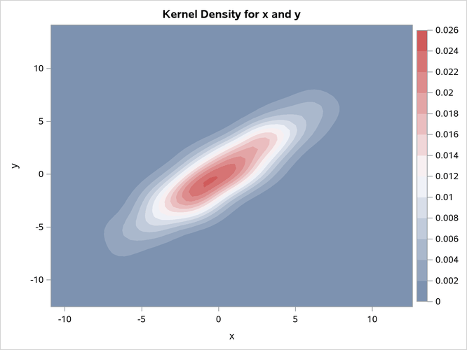
Figure 6: Surface Plot of Estimated Density