Statistical Graphics Using ODS

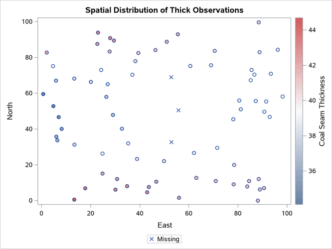
This example is taken from Example 74.2 in Chapter 74, The KRIGE2D Procedure. The coal seam thickness data set is available from the Sashelp library. The following statements create a SAS data set that contains a copy of these data along with some artificially added missing data:

data thick;
   set sashelp.thick;
   if _n_ in (41, 42, 73) then thick = .;
run;

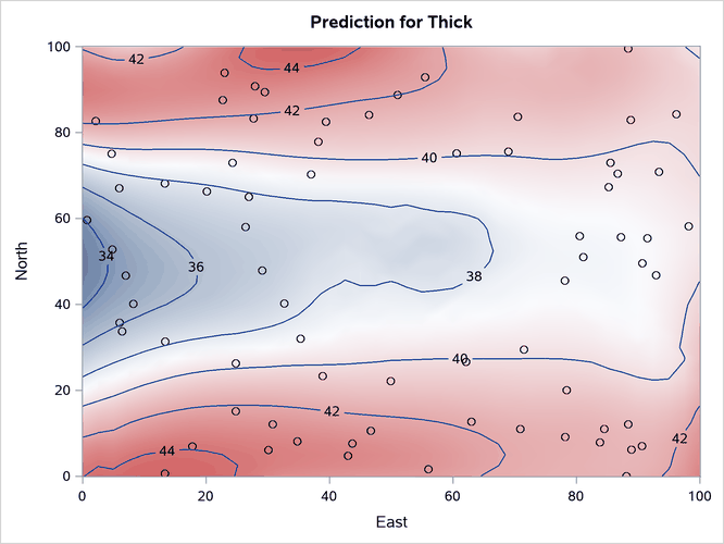
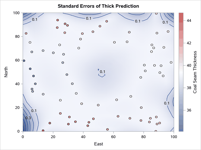
The following statements run PROC KRIGE2D:

proc krige2d data=thick outest=predictions
             plots=(observ(showmissing)
                    pred(fill=pred line=pred obs=linegrad)
                    pred(fill=se line=se obs=linegrad));
   coordinates xc=East yc=North;
   predict var=Thick r=60;
   model scale=7.2881 range=30.6239 form=gauss;
   grid x=0 to 100 by 2.5 y=0 to 100 by 2.5;
run;

The PLOTS=OBSERV(SHOWMISSING) option produces a scatter plot of the data along with the locations of any missing data. The PLOTS=PRED option produces maps of the kriging predictions and standard errors. Two instances of the PLOTS=PRED option are specified along with suboptions that customize the plots. The results are shown in Figure 7.

Figure 7: Spatial Distribution