Statistical Graphics Using ODS
PROC TRANSREG
PROC TRANSREG was the first SAS/STAT modeling procedure to incorporate splines. Its syntax is different from that of other modeling procedures. It predates the EFFECT statement and options in the CLASS statement that other procedures now support.
B-Spline Fit Function
The following step creates a fit plot that has both a classification variable and a spline variable:
proc transreg data=sashelp.gas nomiss solve ss2 plots=fit(nocli noclm);
   ods select anova fitstatistics fitplot;
   model identity(nox) = spline(eqratio / nknots=5 evenly after) |
                         class(fuel / zero=none);
run;
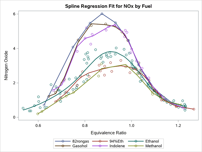
The MODEL statement in PROC TRANSREG lists transformations, expansions, variables, and options. The IDENTITY transformation leaves the dependent variable unchanged. The CLASS expansion replaces the variable Fuel with a set of six binary variables, one for each type of fuel. The vertical bar in the MODEL statement creates an interaction between the SPLINE and CLASS variables. If there were no interaction, the SPLINE transformation would replace the variable EqRatio by a single new variable, which is a linear combination of the columns in a spline basis. Because there is an interaction between the SPLINE and CLASS variables, PROC TRANSREG finds a separate spline transformation for groups of values of the EqRatio variable. There is one group for each level of the CLASS variable (six total).
The model has an implicit intercept, because the ZERO=NONE option creates a binary variable for every level of the CLASS variable. The model has one parameter for each level of the CLASS variable (six total) and eight parameters (degree 3 plus 5 knots) for each spline transformation  total), for a grand total of 54 parameters (53 model df). The AFTER option creates the knots for each term after the SPLINE and CLASS variables are combined to form the interaction term. The structural zeros (those that come from a zero in the binary CLASS variables) are ignored when the knots are found. The EVENLY option spaces the knots evenly; by default, knots are placed at the percentiles. The NOCLI and NOCLM options suppress the default prediction and confidence limits. The results are displayed in Output 24.6.14. Statistical procedures such as PROC TRANSREG display fit statistics in addition to plots. However, PROC TRANSREG does not automatically plot interpolated values. The functions are smoother when there are more data (such as for
 Ethanol) and less smooth for sparser functions (such as 82rongas). The advantage of not interpolating is that the splines are less likely to leave the range of the data.
PROC SGPLOT finds separate fit functions by fitting separate models for each group. In contrast, PROC TRANSREG fits a single model, the one shown previously:

The two approaches are equivalent as long as the knots are the same. However, a procedure such as PROC TRANSREG gives you control over the model beyond anything that PROC SGPLOT gives you. For example, you can force the curves to be the same for each group by omitting the vertical bar from the MODEL statement (in other words, by omitting the interaction of the SPLINE and CLASS variables).
Output 24.6.14: Grouped Fit Function, Fit Statistics, and Plot
| Univariate ANOVA Table Based on the Usual Degrees of Freedom | |||||
|---|---|---|---|---|---|
| Source | DF | Sum of Squares | Mean Square | F Value | Pr > F |
| Model | 53 | 329.1232 | 6.209871 | 64.69 | <.0001 |
| Error | 115 | 11.0388 | 0.095989 | ||
| Corrected Total | 168 | 340.1619 | |||
| Root MSE | 0.30982 | R-Square | 0.9675 |
|---|---|---|---|
| Dependent Mean | 2.34593 | Adj R-Sq | 0.9526 |
| Coeff Var | 13.20676 |
The following example shows how you can set up a data set for interpolation:
proc means data=sashelp.gas(where=(n(nox, eqratio))) noprint;
   class fuel;
   var eqratio;
   output out=m(where=(_type_ eq 1 and trim(_stat_) in ('MIN', 'MAX')));
run;

proc transpose data=m out=m2(drop=_:);
   by fuel;
   id _stat_;
   var eqratio;
run;

data gas(drop=min max);
   if _n_ = 1 then do i = 1 to n;
      set m2 nobs=n point=i;
      if fuel ne '82rongas' then
         do eqratio = min to max by (max - min) / 200; output; end;
   end;
   set sashelp.gas(where=(n(nox, eqratio)));
   output;
run;

proc transreg data=gas solve ss2 plots(interpolate)=fit(nocli noclm);
   ods select anova fitstatistics fitplot;
   model identity(nox) = class(fuel / zero=none) |
                         spline(eqratio / nknots=5 after evenly);
run;
PROC MEANS finds the minimum and maximum for each type of fuel. The WHERE= data set option ensures that only the observations without missing values in the quantitative variables are used. PROC TRANSPOSE arranges the minimum and maximum data set so that there is one observation for each fuel type. The Gas data set adds observations to provide interpolated fit, just as PROC SGPLOT does, except that no interpolated values are generated for the 82rongas group. The results are displayed in Output 24.6.15.
Output 24.6.15: Interpolation
| Univariate ANOVA Table Based on the Usual Degrees of Freedom | |||||
|---|---|---|---|---|---|
| Source | DF | Sum of Squares | Mean Square | F Value | Pr > F |
| Model | 53 | 329.1232 | 6.209871 | 64.69 | <.0001 |
| Error | 115 | 11.0388 | 0.095989 | ||
| Corrected Total | 168 | 340.1619 | |||
| Root MSE | 0.30982 | R-Square | 0.9675 |
|---|---|---|---|
| Dependent Mean | 2.34593 | Adj R-Sq | 0.9526 |
| Coeff Var | 13.20676 |
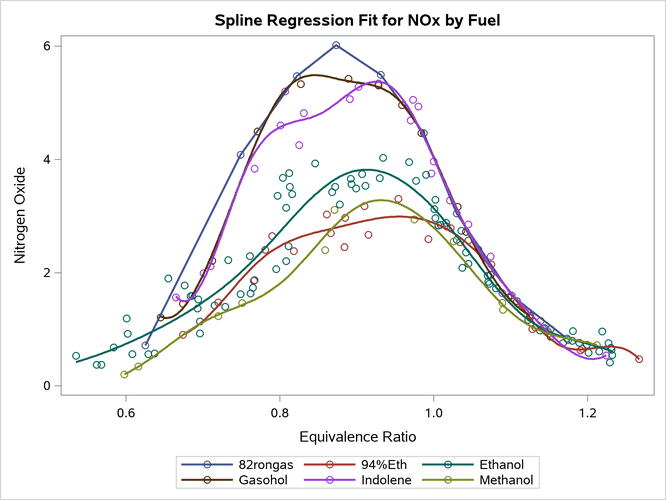
The first PROC TRANSREG step excludes observations that have missing values by using the NOMISS option and analyzes a data set that has 171 observations. The second PROC TRANSREG step excludes observations that have missing values by using a WHERE clause in a preceding DATA step and analyzes a data set that has 1,007 observations. All fit statistics match, because the two data sets contain exactly the same 171 observations that are analyzed. The second data set contains missing values in the variable NOx. Those observations are excluded in IDENTITY transformations. PROC TRANSREG has options for analyzing observations that have missing data, but they are not used for IDENTITY variables. PROC TRANSREG and many other procedures score observations that they exclude from the analysis when computing predicted values, residuals, confidence limits, and so on, as long as the relevant data are there to do the computations, even when those observations are not used in computing the sums of squares, degrees of freedom, coefficients, and so on. The PLOTS(INTERPOLATE) option specifies that those scored observations should be used in plotting the regression functions. When you compare the plots in Output 24.6.14 and Output 24.6.15, you see that the fit functions are the same for 82rongas and are smoother in Output 24.6.15 for the other fuel types.
data gas(drop=min max);
   if _n_ = 1 then do i = 1 to n;
      set m2 nobs=n point=i;
      do eqratio = min to max by (max - min) / 200; output; end;
   end;
   set sashelp.gas(where=(n(nox, eqratio)));
   output;
run;

proc transreg data=gas solve ss2 plots(interpolate)=fit(nocli noclm);
   ods select anova fitstatistics fitplot;
   model identity(nox) = class(fuel / zero=none)
                         spline(eqratio / nknots=5 after evenly);
run;
Parallel Curves
The following steps fit a model without interactions and create the parallel fit functions that are displayed in Output 24.6.16.
Output 24.6.16: Interpolation
| Univariate ANOVA Table Based on the Usual Degrees of Freedom | |||||
|---|---|---|---|---|---|
| Source | DF | Sum of Squares | Mean Square | F Value | Pr > F |
| Model | 13 | 303.1972 | 23.32286 | 97.80 | <.0001 |
| Error | 155 | 36.9647 | 0.23848 | ||
| Corrected Total | 168 | 340.1619 | |||
| Root MSE | 0.48835 | R-Square | 0.8913 |
|---|---|---|---|
| Dependent Mean | 2.34593 | Adj R-Sq | 0.8822 |
| Coeff Var | 20.81676 |
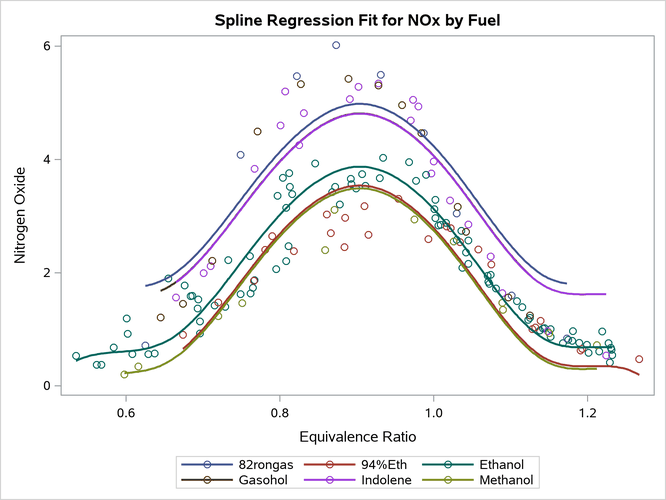
Because the plot has one spline curve and six intercepts, there is no need to guard against the lack of smoothness in the 82rongas fuel type. R-square is smaller in this model because you did not fit a separate curve for each group. You cannot display results like this by using the statistical calculations in PROC SGPLOT; you must first compute the predicted values by using a procedure such as PROC TRANSREG.
Penalized B-Spline Fit Functions
The following step uses penalized B-splines and displays the results in Output 24.6.17:
proc transreg data=gas ss2 plots(interpolate)=fit(nocli noclm);
   ods select anova fitstatistics fitplot;
   model identity(nox) = class(fuel / zero=none) * pbspline(eqratio / after);
run;
Output 24.6.17: Interpolation
| Univariate ANOVA Table, Penalized B-Spline Transformation | |||||
|---|---|---|---|---|---|
| Source | DF | Sum of Squares | Mean Square | F Value | Pr > F |
| Model | 54.288 | 330.1741 | 6.081934 | 69.24 | <.0001 |
| Error | 113.71 | 9.9878 | 0.087834 | ||
| Corrected Total | 168 | 340.1619 | |||
| Root MSE | 0.29637 | R-Square | 0.9706 |
|---|---|---|---|
| Dependent Mean | 2.34593 | Adj R-Sq | 0.9566 |
| Coeff Var | 12.63330 |

The MODEL statement uses an asterisk rather than a vertical bar to specify the interaction. PROC TRANSREG fits multiple types of models. There are linear models such as those shown previously where you can specify either a vertical bar or an asterisk, depending on the type of model that you want. There are also models whose results are computed by preprocessing. For these models, which include penalized B-spline, smoothing spline, and Box-Cox models, you have no freedom to control the intercept terms. Each penalized B-spline has an intercept as part of the model.
Smoothing Spline Functions
PROC TRANSREG has other types of splines, including smoothing splines (Reinsch 1967). This type of spline was first available in PROC GPLOT. The following step fits separate smoothing splines for each fuel and displays the results in Output 24.6.18:
proc transreg data=gas solve ss2 plots(interpolate)=fit(nocli noclm);
   ods select anova fitstatistics fitplot;
   model identity(nox) = class(fuel / zero=none) *
                         smooth(eqratio / after sm=60);
run;
Output 24.6.18: Interpolation
| Univariate ANOVA Table, Smooth Transformation | |||||
|---|---|---|---|---|---|
| Source | DF | Sum of Squares | Mean Square | F Value | Pr > F |
| Model | 29.774 | 322.8643 | 10.84389 | 86.65 | <.0001 |
| Error | 138.23 | 17.2977 | 0.12514 | ||
| Corrected Total | 168 | 340.1619 | |||
| Root MSE | 0.35375 | R-Square | 0.9491 |
|---|---|---|---|
| Dependent Mean | 2.34593 | Adj R-Sq | 0.9382 |
| Coeff Var | 15.07939 |

You use the SM= option to specify a smoothing parameter that ranges from 0 to 100. PROC TRANSREG does not pick an optimal smoothing parameter for you.
Monotone Splines
This example uses artificial data to illustrate monotone splines (Winsberg and Ramsay 1980):
data x;
do i = 1 to 100;
g = 1;
x = 10 * uniform(17);
y = x + 2 * sin(x) + normal(17);
output;
g = 2;
x = 10 * uniform(17);
y = 5 - x - 2 * cos(x) + normal(17);
output;
end;
run;
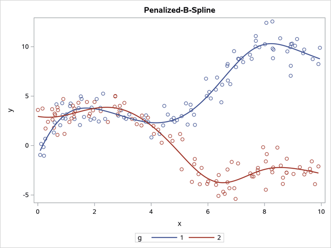
proc sgplot data=x;
title 'Penalized-B-Spline';
pbspline y=y x=x / group=g;
run;
title;
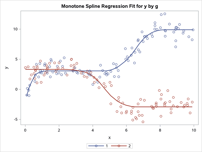
proc transreg data=x ss2 plots=fit(nocli noclm) maxiter=100;
model identity(y) = class(g / zero=none) | mspline(x / nknots=10);
run;
The results are displayed in Output 24.6.19. The first plot, which is produced by PROC SGPLOT, shows the penalized B-spline fit functions, which are not monotonic. The second plot, which is produced by PROC TRANSREG, shows the monotone spline fit functions, which increase for the first group and decrease for the second group. Monotone splines are flat in areas where other splines increase and decrease. A monotone spline transformation of a variable x is always at least weakly increasing (that is, it is increasing or flat). The monotone spline fit function is always (at least weakly) increasing or decreasing, depending on the relationship between y and x. PROC TRANSREG is an iterative procedure. In many cases, you can specify the SOLVE option to directly compute a solution without iterations. However, iterations are required for monotone splines. Monotone splines are quadratic by default (DEGREE=2); most other splines are cubic by default.
Output 24.6.19: Penalized B-Splines and Monotone Splines
Piecewise-Linear Splines
You can specify the option DEGREE=1 along with splines or monotone splines for a piecewise-linear fit function:
proc transreg data=x ss2 plots=fit(nocli noclm) solve;
   model identity(y) = class(g / zero=none) | spline(x / nknots=10 degree=1);
run;

proc transreg data=x ss2 plots=fit(nocli noclm) maxiter=100;
   model identity(y) = class(g / zero=none) | mspline(x / nknots=10 degree=1);
run;
The results are shown in Output 24.6.20.
Output 24.6.20: Piecewise-Linear Splines


Outputting Splines
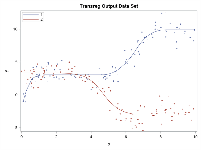
You can create an output data set from a SAS/STAT procedure such as PROC TRANSREG and then use PROC SGPLOT to display the results. This enables you to use the full power of the statistical procedure to fit models and customize the results without modifying a template. The following steps create the plot in Output 24.6.21, which has legend and marker customizations:
proc transreg data=x ss2 plots=fit(nocli noclm) maxiter=100;
   model identity(y) = class(g / zero=none) | mspline(x / nknots=10);
   output out=msp p replace;
run;

proc sort data=msp; by g x; run;

proc sgplot data=msp;
   title 'Transreg Output Data Set';
   scatter y=y  x=x / group=g markerattrs=(size=3px);
   series  y=py x=x / group=g name='a';
   keylegend 'a' / location=inside position=topleft across=1;
run;
title;
Output 24.6.21: Monotone Splines Displayed by PROC SGPLOT