Statistical Graphics Using ODS
B-Splines
This section provides details about how B-splines work and the ways in which you can use them.
Interior and Exterior Knots
Polynomial splines have interior knots (knots that are inside the range of the minimum and maximum x). B-splines have interior knots and exterior knots (knots that are outside the range of the minimum and maximum x). For example, if x ranges from –2 to 2, a reasonable knot vector for three interior knots is  , where
  is a small value such as
  . These knots are all but evenly spaced. The addition and subtraction of ensure that the first three exterior knots are less than the minimum and the last three exterior knots are greater than the maximum. Statistical procedures such as PROC TRANSREG and the procedures that support the EFFECT statement enable you to explicitly control both interior and exterior knots. Simpler options enable you to specify the number of knots and let the procedure determine their values. In many cases, fit functions based on slightly different knots are only slightly different. However, when you fit a model to one set of data and then score another set of data, you must ensure that you use the same knots for both purposes. The following procedure steps all fit the same model and use the knot vector
  :
:
data x2;
   do x = -2 to 2 by 0.1;
      y = x + sin(x) + normal(17);
      output;
   end;
run;

proc transreg data=x2 details ss2;
   model identity(y) = bspline(x / nknots=3 evenly=3);
run;

proc transreg data=x2 details ss2;
   model identity(y) = spline(x / nknots=3 evenly=3);
run;

%let k = -4.000000000001 -3.000000000001 -2.000000000001 -1 0 1
          2.000000000001  3.000000000001  4.000000000001;
proc transreg data=x2 details ss2;
   model identity(y) = bspline(x / knots=&k);
run;

proc orthoreg data=x2;
   effect spl = spline(x / knotmethod=equal(3));
   model  y = spl / noint;
run;

proc orthoreg data=x2;
   effect spl = spline(x / knotmethod=listwithboundary(&k));
   model  y = spl / noint;
run;
Although the models are the same, how the effects are grouped can vary. PROC TRANSREG with the DETAILS option displays the knots shown in Output 24.6.25. PROC TRANSREG with the BSPLINE expansion fits a model that has no intercept and seven 1-df B-spline effects. PROC TRANSREG with the SPLINE transformation fits a model that has an intercept and one 6-df B-spline effect. PROC ORTHOREG fits a model that has no intercept and seven 1-df B-spline effects.
PROC TRANSREG, because it has more than a 30-year history, does not create evenly spaced knots by default. By default, in the data set X2, the knot list is  . (Exterior knots are repeated.) Both repeated and all-but-equally-spaced exterior knots work, but the latter method better matches later software developments.
Output 24.6.25: Interior and Exterior Knots
| Model Statement Specification Details | ||||
|---|---|---|---|---|
| Type | DF | Variable | Description | Value |
| Dep | 1 | Identity(y) | DF | 1 |
| Ind | 6 | Spline(x) | Degree | 3 |
| Number of Knots | 3 | |||
| Exterior Knots | -4.000000000001000E+00 | |||
| -3.000000000001000E+00 | ||||
| -2.000000000001000E+00 | ||||
| Interior Knots | -1.000000000000000E+00 | |||
| 8.8817841970012000E-16 | ||||
| 1.0000000000000000E+00 | ||||
| Exterior Knots | 2.0000000000010000E+00 | |||
| 3.0000000000010000E+00 | ||||
| 4.0000000000010000E+00 | ||||
| Coefficients | -17.07078951 | |||
| 0.20741011 | ||||
| -1.77174923 | ||||
| 0.58192568 | ||||
| 0.54636248 | ||||
| 3.33130267 | ||||
| -8.42096356 | ||||
B-Spline Basis
The following four steps show four equivalent methods of putting the B-spline basis into a SAS data set:
proc transreg data=x2 details ss2;
   model identity(y) = bspline(x / nknots=3 evenly=3);
   output out=b1(keep=x_:) replace;
run;

proc glimmix data=x2 outdesign=b2(drop=x y
   rename=(%macro ren; %do i = 1 %to 7; _x&i=x_%eval(&i-1) %end; %mend; %ren));
   effect spl = spline(x / knotmethod=equal(3));
   model y = spl / noint;
run;

%let k = -4.000000000001 -3.000000000001 -2.000000000001 -1 0 1
          2.000000000001  3.000000000001  4.000000000001;

proc iml;
   use x2(keep=x); read all into x;
   b = bspline(x, 3, {&k});
   vname = 'x_0' : rowcatc('x_' || char(ncol(b)-1));
   create b3 from b[colname=vname]; append from b;
quit;

data b4(keep=x:);
   %let d   = 3;                        /* degree                  */
   %let nkn = %eval(&d * 2 + 3);        /* total number of knots   */
   %let nb  = %eval(&d + 1 + 3);        /* number of cols in basis */
   array k[&nkn] _temporary_ (&k);      /* knots                   */
   array b[&nb] x_0 - x_%eval(&nb - 1); /* basis                   */
   array w[%eval(2 * &d)];              /* work                    */
   set x2;
   do i = 1 to &nb; b[i] = 0; end;

   * find the index of first knot greater than current data value;
   do ki = 1 to &nkn while(k[ki] le x); end;
   kki = ki - &d - 1;

   * make the basis;
   b[1 + kki] = 1;
   do j = 1 to &d;
      w[&d + j] = k[ki + j - 1] - x;
      w[j] = x - k[ki - j];
      s = 0;
      do i = 1 to j;
         t = w[&d + i] + w[j + 1 - i];
         if t ne 0.0 then t = b[i + kki] / t;
         b[i + kki] = s + w[&d + i] * t;
         s = w[j + 1 - i] * t;
      end;
      b[j + 1 + kki] = s;
   end;
run;
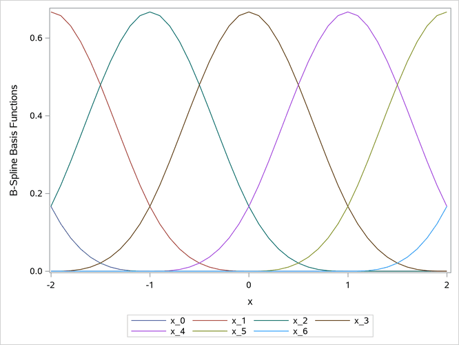
The %REN macro is used to rename the PROC GLIMMIX variables, because different procedures have different rules for naming variables. Each data set has seven columns (intercept, degree 3, and three knots, although no column corresponds directly to these terms). The B-spline basis has at most order 4 (degree + 1) nonzero values in each row. This sparseness can be exploited by modeling code, which is one of the many appealing characteristics of B-splines. The following steps compare and display the bases:
options nolabel;
proc compare error note briefsummary criterion=1e-12
   data=b1 compare=b2 method=relative(1);
run;

proc compare error note briefsummary criterion=1e-12
   data=b1 compare=b3 method=relative(1);
run;

proc compare error note briefsummary criterion=1e-12
   data=b1 compare=b4(drop=x) method=relative(1);
run;
options label;

proc sgplot data=b4;
   %macro s; %do i = 0 %to &nb-1; series y=x_&i x=x; %end; %mend; %s
   yaxis label='B-Spline Basis Functions';
run;
The PROC COMPARE output (not displayed here) shows that the matrices are identical. The B-spline basis is plotted in Output 24.6.26.
Output 24.6.26: B-Spline Basis
The next steps show that the polynomial-spline basis and the B-spline basis are linear transformations of each other:
proc transreg data=x2 details ss2;
   model identity(y) = pspline(x / name=(p) nknots=3);
   output out=p1(keep=p_:) replace;
run;

data both; merge p1 b1; run;

proc print data=both noobs;
   format _numeric_ bestd6.5 p_1 p_2 best6.;
run;

proc cancorr data=both;
  var x:;
  with p:;
run;
The polynomial spline (variables that begin with p_) and B-spline (variables that begin with x_) bases are displayed in Output 24.6.27. The variable p_1 matches the original X variable. All canonical correlations in Output 24.6.28 are 1.0. This shows that every vector in the space that is defined by the columns in the B-spline basis can be constructed from a linear combination of the columns of the polynomial-spline basis.
Output 24.6.27: Polynomial-Spline and B-Spline Bases
| p_1 | p_2 | p_3 | p_4 | p_5 | p_6 | x_0 | x_1 | x_2 | x_3 | x_4 | x_5 | x_6 |
|---|---|---|---|---|---|---|---|---|---|---|---|---|
| -2 | 4 | -8 | 0 | 0 | 0 | 0.1667 | 0.6667 | 0.1667 | 0 | 0 | 0 | 0 |
| -1.9 | 3.61 | -6.859 | 0 | 0 | 0 | 0.1215 | 0.6572 | 0.2212 | 0.0002 | 0 | 0 | 0 |
| -1.8 | 3.24 | -5.832 | 0 | 0 | 0 | 0.0853 | 0.6307 | 0.2827 | 0.0013 | 0 | 0 | 0 |
| -1.7 | 2.89 | -4.913 | 0 | 0 | 0 | 0.0572 | 0.5902 | 0.3482 | 0.0045 | 0 | 0 | 0 |
| -1.6 | 2.56 | -4.096 | 0 | 0 | 0 | 0.0360 | 0.5387 | 0.4147 | 0.0107 | 0 | 0 | 0 |
| -1.5 | 2.25 | -3.375 | 0 | 0 | 0 | 0.0208 | 0.4792 | 0.4792 | 0.0208 | 0 | 0 | 0 |
| -1.4 | 1.96 | -2.744 | 0 | 0 | 0 | 0.0107 | 0.4147 | 0.5387 | 0.0360 | 0 | 0 | 0 |
| -1.3 | 1.69 | -2.197 | 0 | 0 | 0 | 0.0045 | 0.3482 | 0.5902 | 0.0572 | 0 | 0 | 0 |
| -1.2 | 1.44 | -1.728 | 0 | 0 | 0 | 0.0013 | 0.2827 | 0.6307 | 0.0853 | 0 | 0 | 0 |
| -1.1 | 1.21 | -1.331 | 0 | 0 | 0 | 0.0002 | 0.2212 | 0.6572 | 0.1215 | 0 | 0 | 0 |
| -1 | 1 | -1 | 0 | 0 | 0 | 0 | 0.1667 | 0.6667 | 0.1667 | 0 | 0 | 0 |
| -0.9 | 0.81 | -0.729 | 0.0010 | 0 | 0 | 0 | 0.1215 | 0.6572 | 0.2212 | 0.0002 | 0 | 0 |
| -0.8 | 0.64 | -0.512 | 0.0080 | 0 | 0 | 0 | 0.0853 | 0.6307 | 0.2827 | 0.0013 | 0 | 0 |
| -0.7 | 0.49 | -0.343 | 0.0270 | 0 | 0 | 0 | 0.0572 | 0.5902 | 0.3482 | 0.0045 | 0 | 0 |
| -0.6 | 0.36 | -0.216 | 0.0640 | 0 | 0 | 0 | 0.0360 | 0.5387 | 0.4147 | 0.0107 | 0 | 0 |
| -0.5 | 0.25 | -0.125 | 0.1250 | 0 | 0 | 0 | 0.0208 | 0.4792 | 0.4792 | 0.0208 | 0 | 0 |
| -0.4 | 0.16 | -0.064 | 0.2160 | 0 | 0 | 0 | 0.0107 | 0.4147 | 0.5387 | 0.0360 | 0 | 0 |
| -0.3 | 0.09 | -0.027 | 0.3430 | 0 | 0 | 0 | 0.0045 | 0.3482 | 0.5902 | 0.0572 | 0 | 0 |
| -0.2 | 0.04 | -0.008 | 0.5120 | 0 | 0 | 0 | 0.0013 | 0.2827 | 0.6307 | 0.0853 | 0 | 0 |
| -0.1 | 0.01 | -0.001 | 0.7290 | 0 | 0 | 0 | 0.0002 | 0.2212 | 0.6572 | 0.1215 | 0 | 0 |
| 0 | 0 | 0 | 1 | 0 | 0 | 0 | 0 | 0.1667 | 0.6667 | 0.1667 | 0 | 0 |
| 0.1 | 0.01 | 0.0010 | 1.3310 | 0.0010 | 0 | 0 | 0 | 0.1215 | 0.6572 | 0.2212 | 0.0002 | 0 |
| 0.2 | 0.04 | 0.0080 | 1.7280 | 0.0080 | 0 | 0 | 0 | 0.0853 | 0.6307 | 0.2827 | 0.0013 | 0 |
| 0.3 | 0.09 | 0.0270 | 2.1970 | 0.0270 | 0 | 0 | 0 | 0.0572 | 0.5902 | 0.3482 | 0.0045 | 0 |
| 0.4 | 0.16 | 0.0640 | 2.7440 | 0.0640 | 0 | 0 | 0 | 0.0360 | 0.5387 | 0.4147 | 0.0107 | 0 |
| 0.5 | 0.25 | 0.1250 | 3.3750 | 0.1250 | 0 | 0 | 0 | 0.0208 | 0.4792 | 0.4792 | 0.0208 | 0 |
| 0.6 | 0.36 | 0.2160 | 4.0960 | 0.2160 | 0 | 0 | 0 | 0.0107 | 0.4147 | 0.5387 | 0.0360 | 0 |
| 0.7 | 0.49 | 0.3430 | 4.9130 | 0.3430 | 0 | 0 | 0 | 0.0045 | 0.3482 | 0.5902 | 0.0572 | 0 |
| 0.8 | 0.64 | 0.5120 | 5.8320 | 0.5120 | 0 | 0 | 0 | 0.0013 | 0.2827 | 0.6307 | 0.0853 | 0 |
| 0.9 | 0.81 | 0.7290 | 6.8590 | 0.7290 | 0 | 0 | 0 | 0.0002 | 0.2212 | 0.6572 | 0.1215 | 0 |
| 1 | 1 | 1 | 8 | 1 | 0 | 0 | 0 | 0 | 0.1667 | 0.6667 | 0.1667 | 0 |
| 1.1 | 1.21 | 1.3310 | 9.2610 | 1.3310 | 0.0010 | 0 | 0 | 0 | 0.1215 | 0.6572 | 0.2212 | 0.0002 |
| 1.2 | 1.44 | 1.7280 | 10.648 | 1.7280 | 0.0080 | 0 | 0 | 0 | 0.0853 | 0.6307 | 0.2827 | 0.0013 |
| 1.3 | 1.69 | 2.1970 | 12.167 | 2.1970 | 0.0270 | 0 | 0 | 0 | 0.0572 | 0.5902 | 0.3482 | 0.0045 |
| 1.4 | 1.96 | 2.7440 | 13.824 | 2.7440 | 0.0640 | 0 | 0 | 0 | 0.0360 | 0.5387 | 0.4147 | 0.0107 |
| 1.5 | 2.25 | 3.3750 | 15.625 | 3.3750 | 0.1250 | 0 | 0 | 0 | 0.0208 | 0.4792 | 0.4792 | 0.0208 |
| 1.6 | 2.56 | 4.0960 | 17.576 | 4.0960 | 0.2160 | 0 | 0 | 0 | 0.0107 | 0.4147 | 0.5387 | 0.0360 |
| 1.7 | 2.89 | 4.9130 | 19.683 | 4.9130 | 0.3430 | 0 | 0 | 0 | 0.0045 | 0.3482 | 0.5902 | 0.0572 |
| 1.8 | 3.24 | 5.8320 | 21.952 | 5.8320 | 0.5120 | 0 | 0 | 0 | 0.0013 | 0.2827 | 0.6307 | 0.0853 |
| 1.9 | 3.61 | 6.8590 | 24.389 | 6.8590 | 0.7290 | 0 | 0 | 0 | 0.0002 | 0.2212 | 0.6572 | 0.1215 |
| 2 | 4 | 8 | 27 | 8 | 1 | 0 | 0 | 0 | 0 | 0.1667 | 0.6667 | 0.1667 |
Output 24.6.28: Canonical Correlations
| Canonical Correlation |
Adjusted Canonical Correlation |
Approximate Standard Error |
Squared Canonical Correlation |
Eigenvalues of Inv(E)*H = CanRsq/(1-CanRsq) |
Test of H0: The canonical correlations in the current row and all that follow are zero | ||||||||
|---|---|---|---|---|---|---|---|---|---|---|---|---|---|
| Eigenvalue | Difference | Proportion | Cumulative | Likelihood Ratio |
Approximate F Value |
Num DF | Den DF | Pr > F | |||||
| 1 | 1.000000 | . | 0.000000 | 1.000000 | Infty | . | . | . | 0.00000000 | Infty | 36 | 130.11 | <.0001 |
| 2 | 1.000000 | . | 0.000000 | 1.000000 | Infty | . | . | . | 0.00000000 | Infty | 25 | 112.95 | <.0001 |
| 3 | 1.000000 | . | 0.000000 | 1.000000 | Infty | . | . | . | 0.00000000 | Infty | 16 | 95.344 | <.0001 |
| 4 | 1.000000 | . | 0.000000 | 1.000000 | Infty | . | . | . | 0.00000000 | Infty | 9 | 78.03 | <.0001 |
| 5 | 1.000000 | . | 0.000000 | 1.000000 | Infty | . | . | . | 0.00000000 | Infty | 4 | 66 | <.0001 |
| 6 | 1.000000 | . | 0.000000 | 1.000000 | Infty | . | . | 0.00000000 | Infty | 1 | 34 | <.0001 | |