Statistical Graphics Using ODS
Scoring
Many procedures score observations that have missing values or have zero, missing, or invalid weights or frequencies. If the independent variables are all valid, then the procedure can compute predicted values. When the independent and dependent variables are all valid, then the procedure can also compute residuals. The following steps illustrate by using two simple regression models:
data class;
   set sashelp.class(rename=(height=Height1)) nobs=n;
   output;
   if _n_ = n then do;
      call missing(name, sex, height1);
      do age = 10 to 17; output; end;
   end;
run;

proc reg data=class;
   model height1 = age;
   output out=p1 p=p1y r=r1y;
run;

data class;
   f = 1;
   set sashelp.class(rename=(height=Height2)) nobs=n;
   output;
   if _n_ = n then do;
      call missing(f, name, sex);
      do age = 10 to 17; output; end;
   end;
run;

proc reg data=class;
   freq f;
   model height2 = age;
   output out=p2 p=p2y r=r2y;
run;

data all; merge p1 p2; run;

proc print data=all;
   var f name sex age height: p: r:;
   format p1y p2y r1y r2y 6.3;
run;
The results are displayed in Output 24.6.29.
Output 24.6.29: Scoring in a Simple Regression Model
| Obs | f | Name | Sex | Age | Height1 | Height2 | p1y | p2y | r1y | r2y |
|---|---|---|---|---|---|---|---|---|---|---|
| 1 | 1 | Alfred | M | 14 | 69.0 | 69.0 | 64.244 | 64.244 | 4.756 | 4.756 |
| 2 | 1 | Alice | F | 13 | 56.5 | 56.5 | 61.457 | 61.457 | -4.957 | -4.957 |
| 3 | 1 | Barbara | F | 13 | 65.3 | 65.3 | 61.457 | 61.457 | 3.843 | 3.843 |
| 4 | 1 | Carol | F | 14 | 62.8 | 62.8 | 64.244 | 64.244 | -1.444 | -1.444 |
| 5 | 1 | Henry | M | 14 | 63.5 | 63.5 | 64.244 | 64.244 | -0.744 | -0.744 |
| 6 | 1 | James | M | 12 | 57.3 | 57.3 | 58.670 | 58.670 | -1.370 | -1.370 |
| 7 | 1 | Jane | F | 12 | 59.8 | 59.8 | 58.670 | 58.670 | 1.130 | 1.130 |
| 8 | 1 | Janet | F | 15 | 62.5 | 62.5 | 67.031 | 67.031 | -4.531 | -4.531 |
| 9 | 1 | Jeffrey | M | 13 | 62.5 | 62.5 | 61.457 | 61.457 | 1.043 | 1.043 |
| 10 | 1 | John | M | 12 | 59.0 | 59.0 | 58.670 | 58.670 | 0.330 | 0.330 |
| 11 | 1 | Joyce | F | 11 | 51.3 | 51.3 | 55.882 | 55.882 | -4.582 | -4.582 |
| 12 | 1 | Judy | F | 14 | 64.3 | 64.3 | 64.244 | 64.244 | 0.056 | 0.056 |
| 13 | 1 | Louise | F | 12 | 56.3 | 56.3 | 58.670 | 58.670 | -2.370 | -2.370 |
| 14 | 1 | Mary | F | 15 | 66.5 | 66.5 | 67.031 | 67.031 | -0.531 | -0.531 |
| 15 | 1 | Philip | M | 16 | 72.0 | 72.0 | 69.818 | 69.818 | 2.182 | 2.182 |
| 16 | 1 | Robert | M | 12 | 64.8 | 64.8 | 58.670 | 58.670 | 6.130 | 6.130 |
| 17 | 1 | Ronald | M | 15 | 67.0 | 67.0 | 67.031 | 67.031 | -0.031 | -0.031 |
| 18 | 1 | Thomas | M | 11 | 57.5 | 57.5 | 55.882 | 55.882 | 1.618 | 1.618 |
| 19 | 1 | William | M | 15 | 66.5 | 66.5 | 67.031 | 67.031 | -0.531 | -0.531 |
| 20 | . | 10 | . | 66.5 | 53.095 | 53.095 | . | 13.405 | ||
| 21 | . | 11 | . | 66.5 | 55.882 | 55.882 | . | 10.618 | ||
| 22 | . | 12 | . | 66.5 | 58.670 | 58.670 | . | 7.830 | ||
| 23 | . | 13 | . | 66.5 | 61.457 | 61.457 | . | 5.043 | ||
| 24 | . | 14 | . | 66.5 | 64.244 | 64.244 | . | 2.256 | ||
| 25 | . | 15 | . | 66.5 | 67.031 | 67.031 | . | -0.531 | ||
| 26 | . | 16 | . | 66.5 | 69.818 | 69.818 | . | -3.318 | ||
| 27 | . | 17 | . | 66.5 | 72.605 | 72.605 | . | -6.105 |
The first model excludes observations that have missing values. The second model excludes observations that have missing frequencies. The first model uses the variable Height1, which has missing values in the extra observations that are to be scored. The predicted values and residual for the first model are displayed in the variables p1y and r1y, respectively. The second model uses the variable Height2, which has no missing values. The predicted values and residual for the second model are displayed in the variables p1y and r1y, respectively. The predicted values match for both models. The residuals match for the observations that do not have a missing height. For both models, the predicted values for the scored observations match the predicted values for the analysis observations that have the same age. Additionally, the procedure creates predicted values for heights that are not in the data set.
The following steps create observations for each fuel type that are to be scored:
proc means min max data=sashelp.gas;
   class fuel;
   var eqratio;
   output out=m(where=(_type_ eq 1 and _stat_ in ('MIN', 'MAX')));
run;

proc transpose data=m out=m2(drop=_:);
   var eqratio;
   by fuel;
   id _stat_;
run;

data score(drop=min max);
   set m2;
   do eqratio = min to max by (max - min) / 200; output; end;
run;
The following steps concatenate those observations to the data set and use PROC GLIMMIX to score them:
data gas;
   set sashelp.gas(where=(n(nox))) score;
run;

proc glimmix data=gas;
   effect spl = spline(eqratio / naturalcubic knotmethod=equal(5));
   class fuel;
   model nox = spl | fuel;
   output out=scored(where=(nmiss(nox))) pred=py;
run;
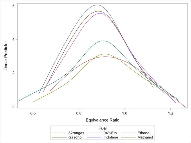
The next step displays the scores:
proc sgplot data=scored;
   series y=py x=eqratio / group=fuel;
run;
Output 24.6.30: Scored Observations
The following steps score the same observations by using the PLM procedure:
proc glimmix data=sashelp.gas;
   effect spl = spline(eqratio / naturalcubic knotmethod=equal(5));
   class fuel;
   model nox = spl | fuel;
   store SplineModel;
run;

proc plm restore=SplineModel;
   score data=score out=scored2 predicted=py;
run;

proc sgplot data=scored2;
   series y=py x=eqratio / group=fuel;
run;
The scores are displayed in Output 24.6.31. For more information about PROC PLM, see Chapter 94, The PLM Procedure.
Output 24.6.31: Observations Scored by PROC PLM
