The PHREG Procedure
Example 92.16 Concordance and ROC Curves
(View the complete code for this example.)
The concordance statistic and ROC curves are popular diagnostic tools for a logistic regression model. For a survival model, ROC curves are time-sensitive. That is, you might have different ROC curves at different time points. Two different ways of computing the concordance statistic are available. Each method estimates a different measure of concordance probability.
The data set Liver, presented in Example 92.12, is used in this example to illustrate the concordance statistic and time-dependent ROC curves. The data set consists of 418 patients who have primary biliary cirrhosis (PBC). In the data set, the variable Time represents the follow-up time in years (which is the time from registration to the earlier of liver transplantation, death, or study termination), the variable Status is the censoring indicator (1 for death and 0 for censored), and the explanatory variables are Age (age in years), Albumin (serum albumin level in g/dl), Bilirubin (serum bilirubin level in mg/dl), Edema (presence of edema), and Protime (prothrombin time in seconds).
The following statements use the PHREG procedure to fit the Cox regression model that uses Bilirubin, Age, and Edema as explanatory variables. The CONCORDANCE option in the PROC PHREG statement requests that Harrell’s concordance statistics be displayed. The PLOTS=ROC option plots the time-dependent ROC curves at time points 2, 4, 6, 8, and 10 years, which are specified in the AT= suboption in the ROCOPTIONS option.
ods graphics on;
proc phreg data=Liver concordance plots=roc rocoptions(at=2 to 10 by 2);
   model Time*Status(0)=Bilirubin Age Edema;
run;
Results of the Harrell concordance statistics are shown in Output 92.16.1. There are 34,798 concordance pairs, 8,884 discordance pairs, 2 pairs that are tied in the linear predictor, and 5 pairs that are tied in the follow-up time, which gives a concordance estimate of 0.7966. You can specify CONCORDANCE=HARRELL(SE) to compute the standard error of Harrell’s concordance statistic, or you can use specify CONCORDANCE=UNO for an alternative concordance measure.
Output 92.16.1: Concordance Statistics
| Harrell's Concordance Statistic | |||||
|---|---|---|---|---|---|
| Source | Estimate | Comparable Pairs | |||
| Concordance | Discordance | Tied in Predictor | Tied in Time | ||
| Model | 0.7966 | 34798 | 8884 | 2 | 5 |
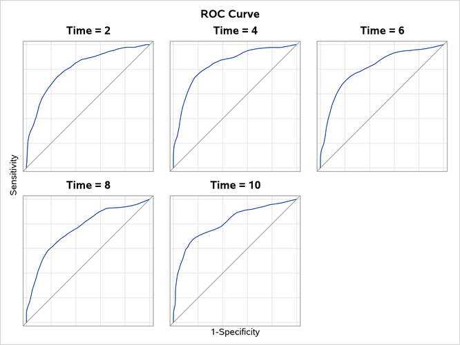
Output 92.16.2 shows the time-dependent ROC curves at the selected years. By default, these curves are computed by the nearest neighbors technique of Heagerty, Lumley, and Pepe (2000) and are displayed in a panel. It appears that among the five selected years, year 4 has the largest area under the curve (AUC), year 8 has the lowest AUC, and the others are in between. If you specify the OVERLAY=INDIVIDUAL global plot option to display individual plots, each plot also displays the area under the ROC curve.
Output 92.16.2: ROC Plot at Selected Time Points
Time-dependent ROC curves change only at the distinct event times. You can examine the area under the curve at all distinct event times by plotting the curve of the AUC. The following statements plot the curve of the AUC of the fitted model and display the 95% pointwise confidence limits. The PLOTS=AUC option in the PROC PHREG statement plots the AUC curve. The ROCOPTIONS in the PROC PHREG statement enables you to specify the inverse probability of censoring weighting (IPCW) method to compute the ROC curves, and the CL suboption requests pointwise confidence limits for the AUC curve.
proc phreg data=Liver plots=auc rocoptions(method=ipcw(cl seed=1234));
   model Time*Status(0)=Bilirubin Age Edema;
run;
Output 92.16.3 displays the AUC curve and the 95% confidence limits for the fitted model. The AUC statistic reaches a high of 0.92 at Year 0.21 but mostly hovers around 0.8.
Output 92.16.3: AUC Plot with 95% Confidence Limits

Consider three submodels of the previously fitted Cox model, each of which contains two of the three covariates: Bilirubin, Age, and Edema. You can use the Uno et al. (2011) methodology to assess the difference of the concordance probabilities between any two submodels. In the following statements, three ROC statements are specified, one for each submodel. The DIFF suboption in CONCORDANCE=UNO in the PROC PHREG statement requests that all pairwise differences be calculated. The SE suboption requests that standard error be computed for each pairwise difference, based on 100 perturbation samples as specified by the ITER= suboption. The seed of the random generator for the perturbation resampling is set to be 1234. The NOFIT option is specified in the MODEL statement, because there is no need to fit the specified model.
proc phreg data=Liver concordance=uno(diff se seed=1234 iter=100);
   model Time*Status(0)=Bilirubin Age Edema / nofit;
   roc 'Bilirubin+Age' Bilirubin Age;
   roc 'Age+Edema' Age Edema;
   roc 'Bilirubin+Edema' Bilirubin Edema;
run;
Output 92.16.4 displays results of the concordance analysis. It appears that the two submodels that contain Bilirubin have a significantly larger concordance probability than the submodel without Bilirubin. In other words, the two submodels that contain Bilirubin predict the survival outcomes better than the model without Bilirubin.
Output 92.16.4: Comparing Uno’s Concordance Estimates
| Differences in Uno's Concordance Statistic | |||||
|---|---|---|---|---|---|
| Source | _Source | Estimate | Standard Error |
Chi-Square | Pr > ChiSq |
| Bilirubin+Age | Age+Edema | 0.0972 | 0.0232 | 17.57 | <.0001 |
| Bilirubin+Age | Bilirubin+Edema | -0.0264 | 0.0231 | 1.31 | 0.2529 |
| Age+Edema | Bilirubin+Edema | -0.1236 | 0.0287 | 18.51 | <.0001 |
Example 92.12 demonstrated that the log transform is a much improved functional form for Bilirubin in a Cox regression model. It is expected that the model with Bilirubin in the log scale would have a better discriminating power than the model with Bilirubin in the original scale. In the following statements, PROC PHREG is used to fit the model with the log transform for Bilirubin. By using the OUTPUT statement, the linear predictor variable is saved as the variable Y in the output data set Liver2. With Liver2 as the input data set, PROC PHREG is called to fit the Cox model with Bilirubin in the original scale. The linear predictor variable Y is specified in the ROC statement as the PRED= variable.
proc phreg data=Liver;
   model Time*Status(0)=logBilirubin Age Edema;
   logBilirubin = log(Bilirubin);
   output out=Liver2 xbeta=Y;
run;
proc phreg data=Liver2 plots=roc rocoptions(at=2 to 10 by 2);
   model Time*Status(0)=Bilirubin Age Edema / roclabel='Bilirubin';
   roc 'logBilirubin' pred=Y;
run;
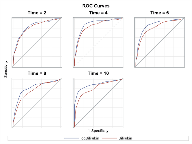
Output 92.16.5 displays the ROC curves of the two competing models. The ROC curve for the model with the log scale for Bilirubin essentially lies above that of its counterpart with the original scale for all the selected time points. This leads to the conclusion that the log transform for Bilirubin improves the predictive power of the model.
Output 92.16.5: ROC Plots to Evaluate the Log Transform for Bilirubin