The PHREG Procedure
Bayesian Analysis
(View the complete code for this example.)
PROC PHREG uses the partial likelihood of the Cox model as the likelihood and generates a chain of posterior distribution samples by the Gibbs Sampler. Summary statistics, convergence diagnostics, and diagnostic plots are provided for each parameter. The following statements generate Figure 4–Figure 10:
ods graphics on;
proc phreg data=Rats;
   model Days*Status(0)=Group;
   bayes seed=1 outpost=Post;
run;
The BAYES statement invokes the Bayesian analysis. The SEED= option is specified to maintain reproducibility; the OUTPOST= option saves the posterior distribution samples in a SAS data set for post-processing; no other options are specified in the BAYES statement. By default, a uniform prior distribution is assumed on the regression coefficient Group. The uniform prior is a flat prior on the real line with a distribution that reflects ignorance of the location of the parameter, placing equal probability on all possible values the regression coefficient can take. Using the uniform prior in the following example, you would expect the Bayesian estimates to resemble the classical results of maximizing the likelihood. If you can elicit an informative prior on the regression coefficients, you should use the COEFFPRIOR= option to specify it.
You should make sure that the posterior distribution samples have achieved convergence before using them for Bayesian inference. PROC PHREG produces three convergence diagnostics by default. If ODS Graphics is enabled before calling PROC PHREG as in the preceding program, diagnostics plots are also displayed.
The results of this analysis are shown in the following figures.
The "Model Information" table in Figure 4 summarizes information about the model you fit and the size of the simulation.
Figure 4: Model Information
| Model Information | ||
|---|---|---|
| Data Set | WORK.RATS | |
| Dependent Variable | Days | Days from Exposure to Death |
| Censoring Variable | Status | |
| Censoring Value(s) | 0 | |
| Model | Cox | |
| Ties Handling | BRESLOW | |
| Sampling Algorithm | ARMS | |
| Burn-In Size | 2000 | |
| MC Sample Size | 10000 | |
| Thinning | 1 | |
PROC PHREG first fits the Cox model by maximizing the partial likelihood. The only parameter in the model is the regression coefficient of Group. The maximum likelihood estimate (MLE) of the parameter and its 95% confidence interval are shown in Figure 5.
Figure 5: Classical Parameter Estimates
| Maximum Likelihood Estimates | |||||
|---|---|---|---|---|---|
| Parameter | DF | Estimate | Standard Error |
95% Confidence Limits | |
| Group | 1 | -0.5959 | 0.3484 | -1.2788 | 0.0870 |
Since no prior is specified for the regression coefficient, the default uniform prior is used. This information is displayed in the "Uniform Prior for Regression Coefficients" table in Figure 6.
Figure 6: Coefficient Prior
| Uniform Prior for Regression Coefficients |
|
|---|---|
| Parameter | Prior |
| Group | Constant |
The "Fit Statistics" table in Figure 7 lists information about the fitted model. The table displays the DIC (deviance information criterion) and pD (effective number of parameters). For more information, see the section Fit Statistics.
Figure 7: Fit Statistics
| Fit Statistics | |
|---|---|
| DIC (smaller is better) | 203.444 |
| pD (Effective Number of Parameters) | 1.003 |
Summary statistics of the posterior samples are displayed in the "Posterior Summaries and Intervals" table in Figure 8. Note that the mean and standard deviation of the posterior samples are comparable to the MLE and its standard error, respectively, because of the use of the uniform prior.
Figure 8: Summary Statistics
| Posterior Summaries and Intervals | |||||
|---|---|---|---|---|---|
| Parameter | N | Mean | Standard Deviation |
95% HPD Interval | |
| Group | 10000 | -0.5998 | 0.3511 | -1.2984 | 0.0756 |
PROC PHREG provides diagnostics to assess the convergence of the generated Markov chain. Figure 9 shows the effective sample size diagnostic. There is no indication that the Markov chain has not reached convergence. For information about interpreting these diagnostics, see the section Statistical Diagnostic Tests in Chapter 8, Introduction to Bayesian Analysis Procedures.
Figure 9: Convergence Diagnostics
| Effective Sample Sizes | |||
|---|---|---|---|
| Parameter | ESS | Autocorrelation Time |
Efficiency |
| Group | 10000.0 | 1.0000 | 1.0000 |
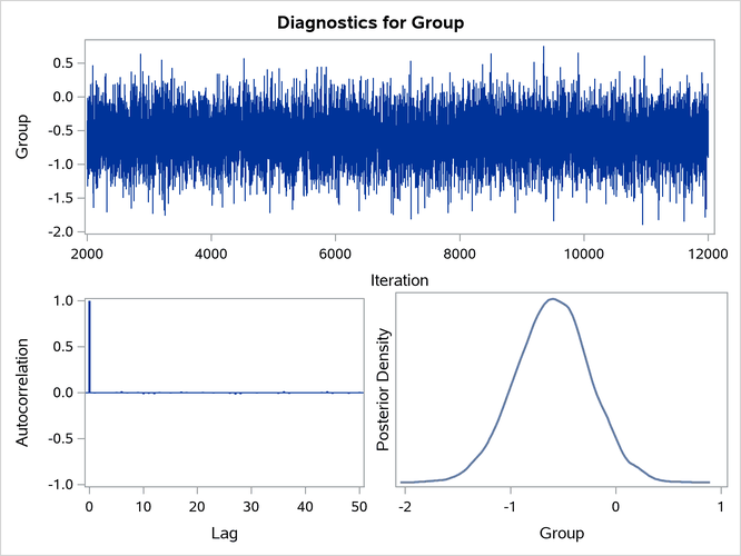
You can also assess the convergence of the generated Markov chain by examining the trace plot, the autocorrelation function plot, and the posterior density plot. Figure 10 displays a panel of these three plots for the parameter Group. This graphical display is automatically produced when ODS Graphics is enabled. Note that the trace of the samples centers on –0.6 with only small fluctuations, the autocorrelations are quite small, and the posterior density appears bell-shaped—all exemplifying the behavior of a converged Markov chain.
Figure 10: Diagnostic Plots
The proportional hazards model for comparing the two pretreatment groups is

The probability that the hazard of Group=0 is greater than that of Group=1 is

This probability can be enumerated from the posterior distribution samples by computing the fraction of samples with a coefficient less than 0. The following DATA step and PROC MEANS perform this calculation:
data New;
   set Post;
   Indicator=(Group < 0);
   label Indicator='Group < 0';
run;
proc means data=New(keep=Indicator) n mean;
run;
Figure 11: Prob(Hazard(Group=0) > Hazard(Group=1))
| Analysis Variable : Indicator Group < 0 |
|
|---|---|
| N | Mean |
| 10000 | 0.9581000 |
The PROC MEANS results are displayed in Figure 11. There is a 95.8% chance that the hazard rate of Group=0 is greater than that of Group=1. The result is consistent with the fact that the average survival time of Group=0 is less than that of Group=1.