The PROBIT Procedure
Estimating the Natural Response Threshold Parameter
(View the complete code for this example.)
Suppose you want to test the effect of a drug at 12 dosage levels. You randomly divide 180 subjects into 12 groups of 15—one group for each dosage level. You then conduct the experiment and, for each subject, record the presence or absence of a positive response to the drug. You summarize the data by counting the number of subjects responding positively in each dose group. Your data set is as follows:
data study;
   input Dose Respond @@;
   Number = 15;
   datalines;
0     3   1.1   4   1.3   4   2.0   3   2.2   5   2.8   4
3.7   5   3.9   9   4.4   8   4.8  11   5.9  12   6.8  13
;
The variable dose represents the amount of drug administered. The first group, receiving a dose level of 0, is the control group. The variable number represents the number of subjects in each group. All groups are equal in size; hence, number has the value 15 for all observations. The variable respond represents the number of subjects responding to the associated drug dosage.
You can model the probability of positive response as a function of dosage by using the following statements:
ods graphics on;

proc probit data=study log10 optc plots=(predpplot ippplot);
   model respond/number=dose;
   output out=new p=p_hat;
run;
The DATA= option specifies that PROC PROBIT analyze the SAS data set study. The LOG10 option replaces the first continuous independent variable (dose) with its common logarithm. The OPTC option estimates the natural response rate. When you use the LOG10 option with the OPTC option, any observations with a dose value less than or equal to zero are used in the estimation as a control group.
The PLOTS= option in the PROC PROBIT statement, together with the ODS GRAPHICS statement, requests two plots for the estimated probability values and dosage levels. For general information about ODS Graphics, see Chapter 24, Statistical Graphics Using ODS. For specific information about the graphics available in the PROBIT procedure, see the section ODS Graphics.
The MODEL statement specifies a proportional response by using the variables respond and number in events/trials syntax. The variable dose is the stimulus or explanatory variable.
The OUTPUT statement creates a new data set, new, that contains all the variables in the original data set, and a new variable, p_hat, that represents the predicted probabilities.
The results from this analysis are displayed in the following figures.
Figure 1 displays background information about the model fit. Included are the name of the input data set, the response variables used, and the number of observations, events, and trials. The last line in Figure 1 shows the final value of the log-likelihood function.
Figure 2 displays the table of parameter estimates for the model. The parameter C, which is the natural response threshold or the proportion of individuals responding at zero dose, is estimated to be 0.2409. Since both the intercept and the slope coefficient have significant p-values (0.0020, 0.0010), you can write the model for

as

where  is the normal cumulative distribution function.
Finally, PROC PROBIT specifies the resulting tolerance distribution by providing the mean MU and scale parameter SIGMA as well as the covariance matrix of the distribution parameters in Figure 3.
Figure 1: Model Fitting Information for the PROBIT Procedure
| Model Information | |
|---|---|
| Data Set | WORK.STUDY |
| Events Variable | Respond |
| Trials Variable | Number |
| Number of Observations | 12 |
| Number of Events | 81 |
| Number of Trials | 180 |
| Number of Events In Control Group | 3 |
| Number of Trials In Control Group | 15 |
| Name of Distribution | Normal |
| Log Likelihood | -104.3945783 |
Figure 2: Model Parameter Estimates for the PROBIT Procedure
| Analysis of Maximum Likelihood Parameter Estimates | |||||||
|---|---|---|---|---|---|---|---|
| Parameter | DF | Estimate | Standard Error |
95% Confidence Limits | Chi-Square | Pr > ChiSq | |
| Intercept | 1 | -4.1438 | 1.3415 | -6.7731 | -1.5146 | 9.54 | 0.0020 |
| Log10(Dose) | 1 | 6.2308 | 1.8996 | 2.5076 | 9.9539 | 10.76 | 0.0010 |
| _C_ | 1 | 0.2409 | 0.0523 | 0.1385 | 0.3433 | ||
Figure 3: Tolerance Distribution Estimates for the PROBIT Procedure
| Estimated Covariance Matrix for Tolerance Parameters | |||
|---|---|---|---|
| MU | SIGMA | _C_ | |
| MU | 0.001158 | -0.000493 | 0.000954 |
| SIGMA | -0.000493 | 0.002394 | -0.000999 |
| _C_ | 0.000954 | -0.000999 | 0.002731 |
The PLOTS=PREDPPLOT option creates the plot in Figure 4, showing the relationship between dosage level, observed response proportions, and estimated probability values. The shaded region is the pointwise confidence band for the fitted probabilities, and a reference line is plotted at the estimated threshold value of 0.24.
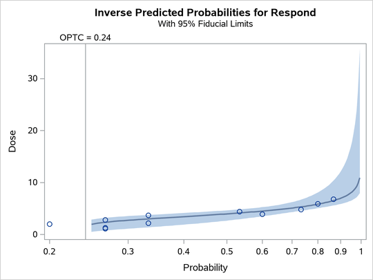
The PLOTS=IPPPLOT option creates the plot in Figure 5, showing the inverse relationship between dosage level and observed response proportions/estimated probability values. The shaded region represents the pointwise fiducial limits for the predicted values of the dose variable, and a reference line is also plotted at the estimated threshold value of 0.24.
The two plot options can be put together with the PLOTS= option, as shown in the PROC PROBIT statement.
Figure 4: Plot of Observed and Fitted Probabilities versus Dose Level
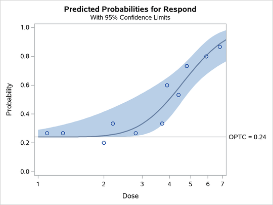
Figure 5: Inverse Predicted Probability Plot with Fiducial Limits