The PSMATCH Procedure
Getting Started: PSMATCH Procedure
(View the complete code for this example.)
This example illustrates the use of the PSMATCH procedure to match observations for individuals in a treatment group with observations for individuals in a control group that have similar propensity scores. The matched observations are saved in an output data set that, with the addition of the outcome variable, can be used to provide an unbiased estimate of the treatment effect.
A pharmaceutical company is conducting a nonrandomized clinical trial to demonstrate the efficacy of a new treatment (Drug_X) by comparing it to an existing treatment (Drug_A). Patients in the trial can choose the treatment that they prefer; otherwise, physicians assign each patient to a treatment. The possibility of treatment selection bias is a concern because it can lead to systematic differences in the distributions of the baseline variables in the two groups, resulting in a biased estimate of treatment effect.
The data set Drugs contains baseline variable measurements for individuals from both treated and control groups. PatientID is the patient identification number, Drug is the treatment group indicator, Gender provides the gender, Age provides the age, and BMI provides the body mass index (a measure of body fat based on height and weight). Typically, more variables are used in a propensity score analysis, but for simplicity only a few variables are used in this example.
Figure 2 lists the first 10 observations.
Figure 2: Input Drug Data Set
| Obs | PatientID | Drug | Gender | Age | BMI |
|---|---|---|---|---|---|
| 1 | 284 | Drug_X | Male | 29 | 22.02 |
| 2 | 201 | Drug_A | Male | 45 | 26.68 |
| 3 | 147 | Drug_A | Male | 42 | 21.84 |
| 4 | 307 | Drug_X | Male | 38 | 22.71 |
| 5 | 433 | Drug_A | Male | 31 | 22.76 |
| 6 | 435 | Drug_A | Male | 43 | 26.86 |
| 7 | 159 | Drug_A | Female | 45 | 25.47 |
| 8 | 368 | Drug_A | Female | 49 | 24.28 |
| 9 | 286 | Drug_A | Male | 31 | 23.31 |
| 10 | 163 | Drug_X | Female | 39 | 25.34 |
Note that the Drugs data set does not contain a response variable, because the response variable is not used in a propensity score analysis. Instead, the response variable is added to the output data set that contains the matched observations, and the combined data set is then used for outcome analysis.
The following statements invoke the PSMATCH procedure and request optimal matching to match observations for patients in the treatment group with observations for patients in the control group:
ods graphics on;
proc psmatch data=drugs region=cs;
   class Drug Gender;
   psmodel Drug(Treated='Drug_X')= Gender Age BMI;
   match method=optimal(k=1) exact=Gender distance=lps caliper=0.25
         weight=none;
   assess lps allcov / plots=(barchart boxplot);
   output out(obs=match)=Outgs lps=_Lps matchid=_MatchID;
run;
The CLASS statement specifies the classification variables. The PSMODEL statement specifies the logistic regression model that creates the propensity score for each observation, which is the probability that the patient receives Drug_X. The Drug variable is the binary treatment indicator variable and TREATED='Drug_X' identifies Drug_X as the treated group. The Gender, Age, and BMI variables are included in the model because they are believed to be related to the assignment.
The REGION= option specifies which observations are used in stratification and matching. In this example, matching is requested by the MATCH statement, and the REGION=CS option requests that only those observations whose propensity scores (or equivalently, logits of propensity scores) lie in the common support region be used for matching. The common support region is defined as the largest interval that contains propensity scores for subjects in both groups. By default, the region is extended by 0.25 times a pooled estimate of the common standard deviation of the logit of the propensity score. For more information, see the description of the EXTEND= option.
The MATCH statement specifies the criteria for matching. The DISTANCE=LPS option (which is the default) requests that the logit of the propensity score be used to compute differences between pairs of observations. The METHOD=OPTIMAL(K=1) option (which is the default) requests optimal matching of one control unit to each unit in the treated group in order to minimize the total within-pair difference, The EXACT=GENDER option forces the treated unit and its matched control unit to have the same value of the Gender variable.
The CALIPER=0.25 option specifies the caliper requirement for matching. This means that for a match to be made, the difference in the logits of the propensity scores for pairs of individuals from the two groups must be less than or equal to 0.25 times the pooled estimate of the common standard deviation of the logits of the propensity scores.
The "Data Information" table in Figure 3 displays information about the input and output data sets, the numbers of observations in the treated and control groups, the lower and upper limits for the propensity score support region, and the numbers of observations in the treated and control groups that fall within the support region. Of the 373 observations in the control group, 351 fall within the support region.
Figure 3: Data Information
| Data Information | |
|---|---|
| Data Set | WORK.DRUGS |
| Output Data Set | WORK.OUTGS |
| Treatment Variable | Drug |
| Treated Group | Drug_X |
| All Obs (Treated) | 113 |
| All Obs (Control) | 373 |
| Support Region | Extended Common Support |
| Lower PS Support | 0.050244 |
| Upper PS Support | 0.683999 |
| Support Region Obs (Treated) | 113 |
| Support Region Obs (Control) | 351 |
The "Propensity Score Information" table in Figure 4 displays summary statistics for propensity scores by treatment group on the basis of all observations, support region observations, and matched observations. When you specify the METHOD=OPTIMAL(K=1) option, all matched observations have the same weight—that is, each matched unit has a weight of 1. Therefore, all the propensity score summary statistics would remain unchanged if you applied these weights to the matched observations. In the example, the WEIGHT=NONE option suppresses the display of summary statistics for weighted matched observations.
Figure 4: Propensity Score Information
| Propensity Score Information | |||||||||||
|---|---|---|---|---|---|---|---|---|---|---|---|
| Observations | Treated (Drug = Drug_X) | Control (Drug = Drug_A) | Treated - Control |
||||||||
| N | Mean | Standard Deviation |
Minimum | Maximum | N | Mean | Standard Deviation |
Minimum | Maximum | Mean Difference |
|
| All | 113 | 0.3108 | 0.1325 | 0.0602 | 0.6411 | 373 | 0.2088 | 0.1320 | 0.0202 | 0.6858 | 0.1020 |
| Region | 113 | 0.3108 | 0.1325 | 0.0602 | 0.6411 | 351 | 0.2176 | 0.1267 | 0.0510 | 0.6824 | 0.0932 |
| Matched | 113 | 0.3108 | 0.1325 | 0.0602 | 0.6411 | 113 | 0.3082 | 0.1310 | 0.0619 | 0.6824 | 0.0025 |
The "Matching Information" table in Figure 5 displays the matching criteria, the number of matched sets, the numbers of matched observations in the treated and control groups, and the total absolute difference in the logit of the propensity score for all matches.
Figure 5: Matching Information
| Matching Information | |
|---|---|
| Distance Metric | Logit of Propensity Score |
| Method | Optimal Fixed Ratio Matching |
| Control/Treated Ratio | 1 |
| Caliper (Logit PS) | 0.191862 |
| Matched Sets | 113 |
| Matched Obs (Treated) | 113 |
| Matched Obs (Control) | 113 |
| Total Absolute Difference | 2.941871 |
The ASSESS statement produces a table and plots that summarize differences in specified variables between treated and control groups. As specified by the LPS and ALLCOV options, these variables are the logit of the propensity score (LPS) and all the covariates in the PSMODEL statement: Gender, Age, and BMI. For a binary classification variable (Gender), the difference is in the proportion of the first ordered level (Female).
The "Standardized Mean Differences" table, shown in Figure 6, displays standardized mean differences for all observations, observations in the support region, and matched observations. The WEIGHT=NONE option suppresses the display of differences for weighted matched observations. Note that when one control unit is matched to each treated unit, the weights are all 1 for matched treated and control units and the results are identical for weighted matched observations and matched observations.
Figure 6: Standardized Mean Differences
| Standardized Mean Differences (Treated - Control) | ||||||
|---|---|---|---|---|---|---|
| Variable | Observations | Mean Difference |
Standard Deviation |
Standardized Difference |
Percent Reduction |
Variance Ratio |
| Logit Prop Score | All | 0.63997 | 0.767449 | 0.83389 | 0.6517 | |
| Region | 0.54546 | 0.71074 | 14.77 | 0.8314 | ||
| Matched | 0.01056 | 0.01375 | 98.35 | 1.0155 | ||
| Age | All | -4.09509 | 6.079104 | -0.67363 | 0.7076 | |
| Region | -3.49368 | -0.57470 | 14.69 | 0.8000 | ||
| Matched | 0.16814 | 0.02766 | 95.89 | 1.1262 | ||
| BMI | All | 0.73930 | 1.923178 | 0.38441 | 0.8854 | |
| Region | 0.63257 | 0.32892 | 14.44 | 0.9288 | ||
| Matched | 0.12425 | 0.06461 | 83.19 | 1.1967 | ||
| Gender | All | -0.02482 | 0.496925 | -0.04994 | 0.9892 | |
| Region | -0.01651 | -0.03323 | 33.46 | 0.9922 | ||
| Matched | 0.00000 | 0.00000 | 100.00 | 1.0000 | ||
| Standard deviation of All observations used to compute standardized differences | ||||||
By default, the standard deviations of the variables, pooled across the treated and control groups, are computed based on all observations. The pooled standard deviations are then used to compute standardized mean differences based on all observations, observations in the support region, and matched observations. You can request a different standard deviation with the STDDEV= option. In Figure 6 the standardized mean differences are significantly reduced in the matched observations. The largest of these differences in absolute value is 0.0646, which is less than the upper limit of 0.25 recommended by Rubin (2001, p. 174) and Stuart (2010, p. 11). However, many authors use an upper limit of 0.10 (Normand et al. 2001; Mamdani et al. 2005; Austin 2009).
The treated-to-control variance ratios between the two groups are between 1 and 1.1967 for all variables in the matched observations, which is within the recommended range of 0.5 to 2 (Rubin 2001, p. 174).
Note that the standardized mean difference for Gender is 0 in the matched observations because EXACT=GENDER is specified in the MATCH statement.
By default, when ODS Graphics is enabled, the PSMATCH procedure displays a standardized mean differences plot for the variables that are specified in the ASSESS statement, as shown in Figure 7.
Figure 7: Standardized Mean Differences Plot
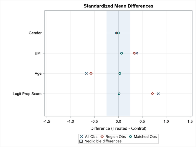
The "Standardized mean Differences Plot" displays the standardized mean differences in the "Standardized Mean Differences" table in Figure 6. All differences for the matched observations are within the recommended limits of –0.25 and 0.25, which are indicated by the shaded area. Again, note that many authors use limits of –0.10 and 0.10. (Normand et al. 2001; Mamdani et al. 2005; Austin 2009). You can use the PLOTS=STDDIFFPLOT(REF=) option to specify the limits for the shaded area.
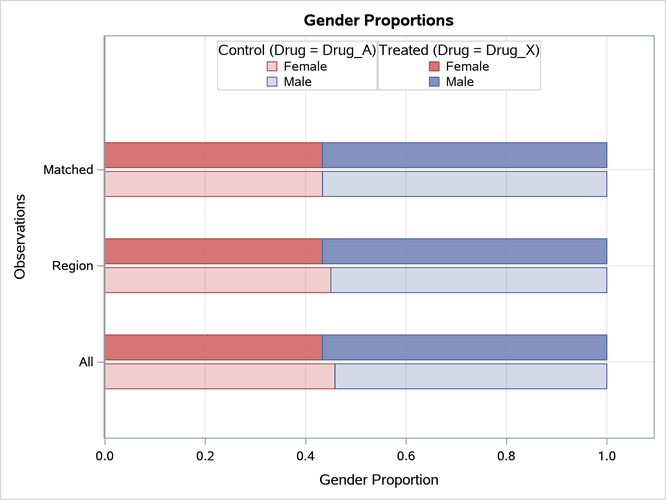
The PLOTS=BARCHART option requests bar charts that compare the treated and control group distributions of binary classification variables that are specified in the ASSESS statement. The bar chart that is created for Gender is shown in Figure 8. The chart displays proportions by default, and it provides comparisons based on all observations, observations in the support region, and matched observations. The distributions of Gender are identical for matched observations because EXACT=GENDER is specified in the MATCH statement.
Figure 8: Gender Bar Chart
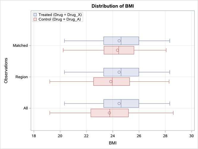
The PLOTS=BOXPLOT option requests box plots for the logit of the propensity score (LPS) and for the continuous variables that are specified in the ASSESS statement, as shown in Figure 9, Figure 10, and Figure 11. The box plots show good variable balance for the matched observations.
Figure 9: LPS Box Plot

Figure 10: Age Box Plot
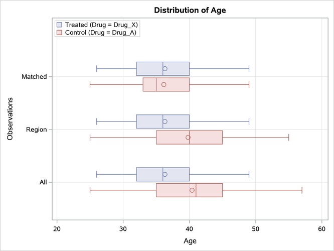
Figure 11: BMI Box Plot
Because the matched observations in this example exhibit good balance, you can output them for subsequent outcome analysis. In situations where you are not satisfied with the balance, you can do one or more of the following to improve the balance: you can select another set of variables for the propensity score model, you can modify the specification of the propensity score model (for example, by introducing nonlinear terms for the continuous variables or by adding interactions), you can modify the matching criteria, or you can choose another matching method.
The OUT(OBS=MATCH)= option in the OUTPUT statement creates an output data set named Outgs that contains the matched observations. By default, this data set includes the variable _PS_ (which provides the propensity score) and the variable _MATCHWGT_ (which provides matched observation weights). The weight for each treated unit is 1. The weight for each matched control unit is also 1 because one control unit is matched to each treated unit. The LPS=_LPS option adds a variable named _LPS that provides the logit of the propensity score, and the MATCHID=_MatchID option adds a variable named _MatchID that identifies the matched sets of observations.
The following statements list the observations in the first five matched sets, as shown in Figure 12.
proc sort data=outgs out=outgs1;
   by _MatchID;
run;

proc print data=outgs1(obs=10);
   var PatientID Drug Gender Age BMI _PS_ _LPS _MatchWgt_ _MatchID;
run;
Figure 12: Output Data Set with Matching Numbers
| Obs | PatientID | Drug | Gender | Age | BMI | _PS_ | _Lps | _MATCHWGT_ | _MatchID |
|---|---|---|---|---|---|---|---|---|---|
| 1 | 213 | Drug_A | Female | 49 | 23.24 | 0.06187 | -2.71892 | 1 | 1 |
| 2 | 89 | Drug_X | Female | 44 | 20.75 | 0.06023 | -2.74745 | 1 | 1 |
| 3 | 141 | Drug_A | Female | 43 | 20.55 | 0.06401 | -2.68256 | 1 | 2 |
| 4 | 323 | Drug_X | Female | 46 | 22.22 | 0.06763 | -2.62375 | 1 | 2 |
| 5 | 420 | Drug_A | Male | 45 | 22.08 | 0.08801 | -2.33814 | 1 | 3 |
| 6 | 217 | Drug_X | Male | 49 | 23.96 | 0.08772 | -2.34185 | 1 | 3 |
| 7 | 234 | Drug_X | Female | 41 | 21.11 | 0.08904 | -2.32538 | 1 | 4 |
| 8 | 290 | Drug_A | Female | 40 | 20.57 | 0.08778 | -2.34104 | 1 | 4 |
| 9 | 320 | Drug_X | Female | 46 | 24.17 | 0.10323 | -2.16184 | 1 | 5 |
| 10 | 473 | Drug_A | Female | 45 | 23.76 | 0.10464 | -2.14670 | 1 | 5 |
After the responses for the trial are observed and added to the matched data set Outgs, you can estimate the treatment effect by carrying out the same type of outcome analysis on Outgs that you would have used with the original data set Drugs (augmented with responses) as if it were a randomized trial (Ho et al. 2007, p. 223). This assumes that no other confounding variables are associated with both the response variable and the treatment group indicator Drug.