The QUANTREG Procedure
Analysis of Fish-Habitat Relationships
(View the complete code for this example.)
Quantile regression is used extensively in ecological studies (Cade and Noon 2003). Recently, Dunham, Cade, and Terrell (2002) applied quantile regression to analyze fish-habitat relationships for Lahontan cutthroat trout in 13 streams of the eastern Lahontan basin, which covers most of northern Nevada and parts of southern Oregon. The density of trout (number of trout per meter) was measured by sampling stream sites from 1993 to 1999. The width-to-depth ratio of the stream site was determined as a measure of stream habitat.
The goal of this study was to explore the relationship between the conditional quantiles of trout density and the width-to-depth ratio. The scatter plot of the data in Figure 1 indicates a nonlinear relationship, so it is reasonable to fit regression models for the conditional quantiles of the log of density. Because regression quantiles are equivariant under any monotonic (linear or nonlinear) transformation (Koenker and Hallock 2001), the exponential transformation converts the conditional quantiles to the original density scale.
The data set trout, which follows, includes the average numbers of Lahontan cutthroat trout per meter of stream (Density), the logarithm of Density (LnDensity), and the width-to-depth ratios (WDRatio) for 71 samples:
data trout;
   input Density WDRatio LnDensity @@;
   datalines;
 0.38732     8.6819    -0.94850    1.16956    10.5102     0.15662
 0.42025    10.7636    -0.86690    0.50059    12.7884    -0.69197
 0.74235    12.9266    -0.29793    0.40385    14.4884    -0.90672
 0.35245    15.2476    -1.04284    0.11499    16.6495    -2.16289
 0.18290    16.7188    -1.69881    0.06619    16.7859    -2.71523
 0.70330    19.0141    -0.35197    0.50845    19.0548    -0.67639

   ... more lines ...

 0.25125    54.6916    -1.38129
;
The following statements use the QUANTREG procedure to fit a simple linear model for the 50th and 90th percentiles of LnDensity:
ods graphics on;

proc quantreg data=trout alpha=0.1 ci=resampling;
   model LnDensity = WDRatio / quantile=0.5 0.9
                               CovB seed=1268;
   test WDRatio / wald lr;
run;
The MODEL statement specifies a simple linear regression model with LnDensity as the response variable Y and WDRatio as the covariate X. The QUANTILE= option requests that the regression quantile function  be estimated by solving the following equation, where
  :
:

By default, the regression coefficients  are estimated by using the simplex algorithm, which is explained in the section Simplex Algorithm. The ALPHA= option requests 90% confidence limits for the regression parameters, and the option CI=RESAMPLING specifies that the intervals be computed by using the Markov chain marginal bootstrap (MCMB) resampling method of He and Hu (2002). When you specify the CI=RESAMPLING option, the QUANTREG procedure also computes standard errors, t values, and p-values of regression parameters by using the MCMB resampling method. The SEED= option specifies a seed for the resampling method. The COVB option requests covariance matrices for the estimated regression coefficients, and the TEST statement requests tests for the hypothesis that the slope parameter (the coefficient of
 WDRatio) is 0.
Figure 3 displays model information and summary statistics for the variables in the model. The summary statistics include the median and the standardized median absolute deviation (MAD), which are robust measures of univariate location and scale, respectively. For more information about the standardized MAD, see Huber (1981, p. 108).
Figure 3: Model Fitting Information and Summary Statistics
| Model Information | |
|---|---|
| Data Set | WORK.TROUT |
| Dependent Variable | LnDensity |
| Number of Independent Variables | 1 |
| Number of Observations | 71 |
| Optimization Algorithm | Simplex |
| Method for Confidence Limits | Resampling |
| Quantile Levels | 2 |
| Summary Statistics | ||||||
|---|---|---|---|---|---|---|
| Variable | Q1 | Median | Q3 | Mean | Standard Deviation |
MAD |
| WDRatio | 22.0917 | 29.4083 | 35.9382 | 29.1752 | 9.9859 | 10.4970 |
| LnDensity | -2.0511 | -1.3813 | -0.8669 | -1.4973 | 0.7682 | 0.8214 |
Figure 4 and Figure 5 display the parameter estimates, standard errors, 95% confidence limits, t values, and p-values that are computed by the resampling method.
Figure 4: Parameter Estimates at QUANTILE=0.5
| Parameter Estimates | |||||||
|---|---|---|---|---|---|---|---|
| Parameter | DF | Estimate | Standard Error |
90% Confidence Limits | t Value | Pr > |t| | |
| Intercept | 1 | -0.9811 | 0.3952 | -1.6400 | -0.3222 | -2.48 | 0.0155 |
| WDRatio | 1 | -0.0136 | 0.0123 | -0.0341 | 0.0068 | -1.11 | 0.2705 |
Figure 5: Parameter Estimates at QUANTILE=0.9
| Parameter Estimates | |||||||
|---|---|---|---|---|---|---|---|
| Parameter | DF | Estimate | Standard Error |
90% Confidence Limits | t Value | Pr > |t| | |
| Intercept | 1 | 0.0576 | 0.2606 | -0.3769 | 0.4921 | 0.22 | 0.8257 |
| WDRatio | 1 | -0.0215 | 0.0075 | -0.0340 | -0.0091 | -2.88 | 0.0053 |
The 90th percentile of trout density can be predicted from the width-to-depth ratio as follows:

This is the upper dashed curve that is plotted in Figure 1. The lower dashed curve for the median can be obtained in a similar fashion.
The covariance matrices for the estimated parameters are shown in Figure 6. The resampling method that is used for the confidence intervals is also used to compute these matrices.
Figure 6: Covariance Matrices of the Estimated Parameters
| Estimated Covariance Matrix for Quantile Level = 0.5 |
||
|---|---|---|
| Intercept | WDRatio | |
| Intercept | 0.156191 | -.004653 |
| WDRatio | -.004653 | 0.000151 |
| Estimated Covariance Matrix for Quantile Level = 0.9 |
||
|---|---|---|
| Intercept | WDRatio | |
| Intercept | 0.067914 | -.001877 |
| WDRatio | -.001877 | 0.000056 |
The tests requested by the TEST statement are shown in Figure 7. Both the Wald test and the likelihood ratio test indicate that the coefficient of width-to-depth ratio is significantly different from 0 at the 90th percentile, but the difference is not significant at the median.
Figure 7: Tests of Significance
| Test Results | |||||
|---|---|---|---|---|---|
| Quantile Level |
Test | Test Statistic |
DF | Chi-Square | Pr > ChiSq |
| 0.5 | Wald | 1.2339 | 1 | 1.23 | 0.2666 |
| 0.5 | Likelihood Ratio | 1.1467 | 1 | 1.15 | 0.2842 |
| 0.9 | Wald | 8.3031 | 1 | 8.30 | 0.0040 |
| 0.9 | Likelihood Ratio | 9.0529 | 1 | 9.05 | 0.0026 |
In many quantile regression problems it is useful to examine how the estimated regression parameters for each covariate change as a function of  in the interval
  . The following statements use the QUANTREG procedure to request the estimated quantile processes
  for the slope and intercept parameters:
proc quantreg data=trout alpha=0.1 ci=resampling;
   model LnDensity = WDRatio / quantile=process seed=1268
                               plot=quantplot;
run;
The QUANTILE=PROCESS option requests an estimate of the quantile process for each regression parameter. The options ALPHA=0.1 and CI=RESAMPLING specify that 90% confidence bands for the quantile processes be computed by using the resampling method.
Figure 8 displays a portion of the objective function table for the quantile process model. The objective function is evaluated at 77 values of in the interval . The table also provides predicted values of the conditional quantile function  at the mean for
 WDRatio, which can be used to estimate the conditional density function.
Figure 8: Objective Function Values for Quantile Process
| Objective Function for Quantile Process |
|||
|---|---|---|---|
| Label | Quantile Level |
Objective Function |
Predicted at Mean |
| t0 | 0.005634 | 0.7044 | -3.2582 |
| t1 | 0.020260 | 2.5331 | -3.0331 |
| t2 | 0.031348 | 3.7421 | -2.9376 |
| t3 | 0.046131 | 5.2538 | -2.7013 |
| . | . | . | . |
| . | . | . | . |
| . | . | . | . |
| t73 | 0.945705 | 4.1433 | -0.4361 |
| t74 | 0.966377 | 2.5858 | -0.4287 |
| t75 | 0.976060 | 1.8512 | -0.4082 |
| t76 | 0.994366 | 0.4356 | -0.4082 |
Figure 9 displays a portion of the table of the quantile processes for the estimated parameters and confidence limits.
Figure 9: Parameter Estimates for Quantile Process
| Parameter Estimates for Quantile Process | |||
|---|---|---|---|
| Label | Quantile Level |
Intercept | WDRatio |
| . | . | . | . |
| . | . | . | . |
| . | . | . | . |
| t57 | 0.765705 | -0.42205 | -0.01335 |
| lower90 | 0.765705 | -0.91952 | -0.02682 |
| upper90 | 0.765705 | 0.07541 | 0.00012 |
| t58 | 0.786206 | -0.32688 | -0.01592 |
| lower90 | 0.786206 | -0.80883 | -0.02895 |
| upper90 | 0.786206 | 0.15507 | -0.00289 |
| . | . | . | . |
| . | . | . | . |
| . | . | . | . |
When ODS Graphics is enabled, the PLOT=QUANTPLOT option in the MODEL statement requests a plot of the estimated quantile processes.
For more information about enabling and disabling ODS Graphics, see the section Enabling and Disabling ODS Graphics in Chapter 24, Statistical Graphics Using ODS.
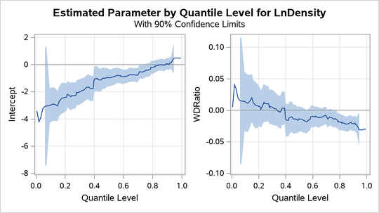
The left side of Figure 10 displays the process for the intercept, and the right side displays the process for the coefficient of WDRatio.
The process plot for WDRatio shows that the slope parameter changes from positive to negative as the quantile increases and that it changes sign with a sharp drop at the 40th percentile. The 90% confidence bands show that the relationship between LnDensity and WDRatio (expressed by the slope) is not significant below the 78th percentile. This situation can also be seen in Figure 9, which shows that 0 falls between the lower and upper confidence limits of the slope parameter for quantiles below 0.78. Since the confidence intervals for the extreme quantiles are not stable because of insufficient data, the confidence band is not displayed outside the interval (0.05, 0.95).
Figure 10: Quantile Processes for Intercept and Slope
The QUANTILE=FQPR(N=q) option performs parameter estimation for the quantile process model in the equally spaced quantile-level grid  by using the fast quantile process regression algorithm. The following statements estimate the quantile process model,
  , in a size-100, equally spaced quantile-level grid:
ods output ProcessEst=oProEst;
proc quantreg data=trout ci=none;
   model LnDensity = WDRatio / quantile=fqpr(n=100);
run;
Figure 11 displays a portion of the table that shows the parameter estimates of the quantile process model.
Figure 11: Parameter Estimates for Quantile Process
| Parameter Estimates for Quantile Process | |||
|---|---|---|---|
| Label | Quantile Level |
Intercept | WDRatio |
| t0 | 0.005000 | -3.39929 | 0.00483 |
| t1 | 0.015000 | -3.39929 | 0.00483 |
| t2 | 0.025000 | -4.21355 | 0.04046 |
| t3 | 0.035000 | -3.94081 | 0.03439 |
| t4 | 0.045000 | -3.94081 | 0.03439 |
| t5 | . | . | . |
| t99 | 0.995000 | 0.47468 | -0.03026 |
Figure 12 displays the information about the quantile-level grid, the average objective-function value, and the average prediction at the mean value of WDRatio.
Figure 12: Average Objective Function
| Quantile Levels and Average Objective Function | |
|---|---|
| Number of Quantile Levels | 100 |
| Minimum Quantile Level | 0.0050 |
| Maximum Quantile Level | 0.9950 |
| Average Objective Function | 15.0539 |
| Average Predicted Value at Mean | -1.4989 |
Figure 13 displays the average parameter estimates that model the conditional mean of the response variable LnDensity and are comparable to the parameter estimates from its counterpart linear regression model.
Figure 13: Average Parameter Estimates
| Average Parameter Estimates | ||
|---|---|---|
| Parameter | DF | Estimate |
| Intercept | 1 | -1.3307 |
| WDRatio | 1 | -0.0058 |
You can perform observationwise conditional distribution analysis by using the quantile process model. The following statements sort all the observations in ascending order of the width-to-depth ratios (WDRatio), and they use the CONDDIST statement of the QUANTREG procedure to perform the conditional distribution analysis for the second, 15th, 37th, and 63rd observations:
proc sort data=trout;
   by WDRatio;
run;

proc quantreg data=trout ci=none;
   model LnDensity = WDRatio / quantile=fqpr(n=100);
   conddist hr obs= 2 15 37 63 plots=all;
run;
Figure 14 displays the four selected training observations under conditional distribution analysis.
Figure 14: Observations for Conditional Distribution Analysis
| Observations for Conditional Distribution Analysis |
|||
|---|---|---|---|
| Label | Logarithm of Density |
Density | WDRatio |
| 2 | 0.15662 | 1.16956 | 10.5102 |
| 15 | -1.35772 | 0.25725 | 20.7852 |
| 37 | -0.58719 | 0.55589 | 30.9569 |
| 63 | -1.52685 | 0.21722 | 40.0388 |
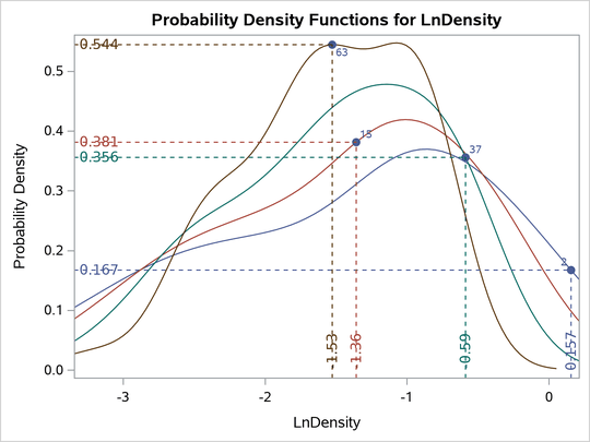
Figure 15 shows the conditional distribution estimates for the selected observations. In Figure 15, the regression quantile levels measure the quantile levels (which are equivalent to percentages) of the response values conditional on their respective WDRatio values; the sample quantile levels measure the percentages of the same response values in the pool of all the training response values without adjustment on their respective WDRatio values.
Figure 15: Average Objective Function
| Conditional Distribution Estimates | ||||||
|---|---|---|---|---|---|---|
| Data | Type | Label | Response Value |
Quantile Level | Regression Density |
|
| Regression | Sample | |||||
| Training | Fit for Obs | 2 | 0.156620 | 0.9873 | 0.9930 | 0.167156 |
| Training | Fit for Obs | 15 | -1.35772 | 0.4325 | 0.5141 | 0.381070 |
| Training | Fit for Obs | 37 | -0.58719 | 0.9350 | 0.9225 | 0.355702 |
| Training | Fit for Obs | 63 | -1.52685 | 0.5345 | 0.4155 | 0.544205 |
Figure 16 and Figure 17, respectively, show the cumulative distribution functions (CDFs) and the probability density functions (PDFs) of the response random variables for the four selected observations conditional on their respective WDRatio values. The dots represent the observed response values of the selected observations on the X axis, the relevant regression quantile levels on the Y axis (in Figure 16), and the relevant probability density values on the Y axis (in Figure 17).
Figure 16: Conditional CDFs for the Selected Observations
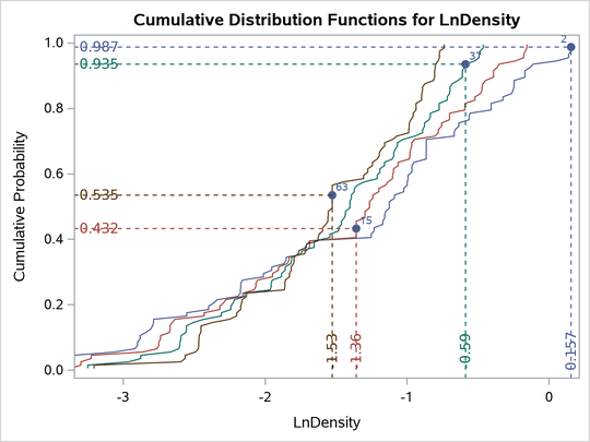
Figure 17: Conditional PDFs for the Selected Observations