The SEQDESIGN Procedure
Example 110.8 Creating a One-Sided Error Spending Design
(View the complete code for this example.)
This example requests a five-stage, one-sided group sequential design for normally distributed statistics. The design uses an O’Brien-Fleming-type error spending function for the  boundary and a Pocock-type error spending function for the
  boundary. The following statements request a one-sided design by using different and spending functions:
ods graphics on;
proc seqdesign altref=0.2  errspend
               pss(cref=0 0.5 1)
               stopprob(cref=0 0.5 1)
               plots=(asn power errspend)
               ;
   OneSidedErrorSpending: design nstages=5
                          method(alpha)=errfuncobf
                          method(beta)=errfuncpoc
                          alt=upper  stop=both
                          alpha=0.025
                          ;
run;
The "Design Information" table in Output 110.8.1 displays design specifications and the derived statistics. With the specified alternative reference, the maximum information is derived.
Output 110.8.1: Error Spending Method Design Information
| Design Information | |
|---|---|
| Statistic Distribution | Normal |
| Boundary Scale | Standardized Z |
| Alternative Hypothesis | Upper |
| Early Stop | Accept/Reject Null |
| Method | Error Spending |
| Boundary Key | Both |
| Alternative Reference | 0.2 |
| Number of Stages | 5 |
| Alpha | 0.025 |
| Beta | 0.1 |
| Power | 0.9 |
| Max Information (Percent of Fixed Sample) | 119.4278 |
| Max Information | 313.7196 |
| Null Ref ASN (Percent of Fixed Sample) | 50.35408 |
| Alt Ref ASN (Percent of Fixed Sample) | 78.77223 |
The "Method Information" table in Output 110.8.2 displays the and errors, alternative reference, and derived drift parameter, which is the standardized alternative reference at the final stage.
Output 110.8.2: Method Information
| Method Information | ||||||
|---|---|---|---|---|---|---|
| Boundary | Method | Alpha | Beta | Error Spending | Alternative Reference |
Drift |
| Function | ||||||
| Upper Alpha | Error Spending | 0.02500 | . | Approx O'Brien-Fleming | 0.2 | 3.542426 |
| Upper Beta | Error Spending | . | 0.10000 | Approx Pocock | 0.2 | 3.542426 |
With the STOPPROB option, the "Expected Cumulative Stopping Probabilities" table in Output 110.8.3 displays the expected stopping stage and cumulative stopping probability to reject the null hypothesis at each stage under various hypothetical references  , where
  is the alternative reference and
  are values specified in the CREF= option.
Output 110.8.3: Stopping Probabilities
| Expected Cumulative Stopping Probabilities Reference = CRef * (Alt Reference) |
|||||||
|---|---|---|---|---|---|---|---|
| CRef | Expected Stopping Stage |
Source | Stopping Probabilities | ||||
| Stage_1 | Stage_2 | Stage_3 | Stage_4 | Stage_5 | |||
| 0.0000 | 2.108 | Reject Null | 0.00000 | 0.00039 | 0.00381 | 0.01221 | 0.02500 |
| 0.0000 | 2.108 | Accept Null | 0.38080 | 0.69133 | 0.86162 | 0.94170 | 0.97500 |
| 0.0000 | 2.108 | Total | 0.38080 | 0.69173 | 0.86543 | 0.95391 | 1.00000 |
| 0.5000 | 3.296 | Reject Null | 0.00002 | 0.01265 | 0.09650 | 0.24465 | 0.38724 |
| 0.5000 | 3.296 | Accept Null | 0.13665 | 0.28063 | 0.41080 | 0.52230 | 0.61276 |
| 0.5000 | 3.296 | Total | 0.13667 | 0.29328 | 0.50730 | 0.76695 | 1.00000 |
| 1.0000 | 3.298 | Reject Null | 0.00050 | 0.13209 | 0.52642 | 0.80390 | 0.90000 |
| 1.0000 | 3.298 | Accept Null | 0.02954 | 0.05231 | 0.07085 | 0.08648 | 0.10000 |
| 1.0000 | 3.298 | Total | 0.03004 | 0.18440 | 0.59728 | 0.89039 | 1.00000 |
With the PSS option, the "Power and Expected Sample Sizes" table in Output 110.8.4 displays powers and expected sample sizes under various hypothetical references , where is the alternative reference and  are the default values in the CREF= option.
Output 110.8.4: Power and Expected Sample Size Information
| Powers and Expected Sample Sizes Reference = CRef * (Alt Reference) |
||
|---|---|---|
| CRef | Power | Sample Size |
| Percent Fixed-Sample |
||
| 0.0000 | 0.02500 | 50.3541 |
| 0.5000 | 0.38724 | 78.7219 |
| 1.0000 | 0.90000 | 78.7722 |
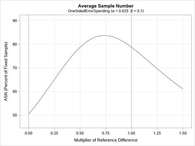
With the PLOTS=ASN option, the procedure displays a plot of expected sample sizes under various hypothetical references, as shown in Output 110.8.5. By default, expected sample sizes under the hypotheses  ,
,  , are displayed, where is the alternative reference.
Output 110.8.5: ASN Plot
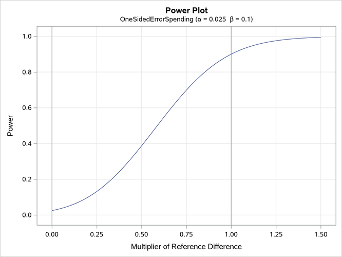
With the PLOTS=POWER option, the procedure displays a plot of the power curves under various hypothetical references for all designs simultaneously, as shown in Output 110.8.6. By default, the option CREF=  and powers under hypothetical references are displayed, where are values specified in the CREF= option. These CREF= values are displayed on the horizontal axis.
Under the null hypothesis,  , the power is 0.025, the upper Type I error probability. Under the alternative hypothesis,
  , the power is 0.9, one minus the Type II error probability. The plot shows only minor difference between the two designs.
Output 110.8.6: Power Plot
The "Boundary Information" table in Output 110.8.7 displays information level, alternative reference, and boundary values. By default (or equivalently if you specify BOUNDARYSCALE=STDZ), the alternative reference and boundary values are displayed with the standardized Z scale. That is, the resulting standardized alternative reference at stage k is given by  , where
  is the specified alternative reference and
  is the information level at stage k,
  .
.
Output 110.8.7: Boundary Information
| Boundary Information (Standardized Z Scale) Null Reference = 0 |
|||||
|---|---|---|---|---|---|
| _Stage_ | Alternative | Boundary Values | |||
| Information Level | Reference | Upper | |||
| Proportion | Actual | Upper | Beta | Alpha | |
| 1 | 0.2000 | 62.74393 | 1.58422 | -0.30338 | 4.87688 |
| 2 | 0.4000 | 125.4879 | 2.24043 | 0.41667 | 3.35706 |
| 3 | 0.6000 | 188.2318 | 2.74395 | 0.97165 | 2.67766 |
| 4 | 0.8000 | 250.9757 | 3.16844 | 1.43627 | 2.26535 |
| 5 | 1.0000 | 313.7196 | 3.54243 | 1.87522 | 1.87522 |
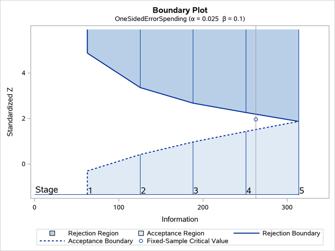
With ODS Graphics enabled, a detailed boundary plot with the rejection and acceptance regions is displayed, as shown in Output 110.8.8. This plot displays the boundary values in the "Boundary Information" table in Output 110.8.7.
Output 110.8.8: Boundary Plot
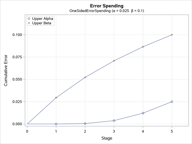
The "Error Spending Information" table in Output 110.8.9 displays cumulative error spending at each stage for each boundary.
Output 110.8.9: Error Spending Information
| Error Spending Information | |||
|---|---|---|---|
| _Stage_ | Information Level |
Cumulative Error Spending | |
| Upper | |||
| Proportion | Beta | Alpha | |
| 1 | 0.2000 | 0.02954 | 0.00000 |
| 2 | 0.4000 | 0.05231 | 0.00039 |
| 3 | 0.6000 | 0.07085 | 0.00381 |
| 4 | 0.8000 | 0.08648 | 0.01221 |
| 5 | 1.0000 | 0.10000 | 0.02500 |
With the PLOTS=ERRSPEND option, the procedure displays a plot of error spending for each boundary, as shown in Output 110.8.10. This plot displays the cumulative error spending at each stage in the "Error Spending Information" table in Output 110.8.9. The O’Brien-Fleming-type spending function is conservative in early stages because it uses much less at early stages than in the later stages. In contrast, the Pocock-type spending function uses more at early stages than in the later stages.
Output 110.8.10: Error Spending Plot