The SURVEYFREQ Procedure
Getting Started: SURVEYFREQ Procedure
(View the complete code for this example.)
The following example shows how to use PROC SURVEYFREQ to construct and analyze frequency tables from sample survey data. This example uses simulated data from a customer satisfaction survey for a student information system (SIS).
Suppose a company conducted a survey of school personnel who use the SIS, which is a software product that provides modules for student registration, class scheduling, attendance, grade reporting, and other functions. A probability sample of SIS users was selected from the study population, which included SIS users at middle schools and high schools in the states of Georgia, South Carolina, and North Carolina. The sample design for this survey was a two-stage stratified design. A first-stage sample of schools was selected from the list of schools in the three states that use the SIS. The list of schools, which are the primary sampling units (PSU), was stratified by state and by customer status (whether the school was a new user or a renewal user of the system). Within the strata, schools were selected with probability proportional to size and with replacement, where the size measure was school enrollment. From each sample school, five staff members were randomly selected with replacement as the second-stage sample to complete the SIS satisfaction questionnaire.
The SAS data set SIS_Survey contains the survey results and the sample design information that is needed to analyze the data. This data set contains the following variables:
State: state where the school is locatedNewUser: 'New Customer' or 'Renewal Customer'School: school identification (PSU)SchoolType: 'High School' or 'Middle School'Department: 'Faculty' or 'Admin/Guidance'SamplingWeight: sampling weightResponse: response, from "Very Unsatisfied" to "Very Satisfied"
The variables State and NewUser identify the first-stage strata from which schools were selected. The variable School identifies the primary sampling units (clusters). The variable SamplingWeight contains the sampling weight for each respondent. Sampling weights were computed from the selection probabilities at each stage of sampling and were adjusted for nonresponse.
The following PROC SURVEYFREQ statements request a one-way frequency table for the variable Response:
title 'Student Information System Survey';
proc surveyfreq data=SIS_Survey;
   tables  Response;
   strata  State NewUser;
   cluster School;
   weight  SamplingWeight;
run;
The PROC SURVEYFREQ statement invokes the procedure and identifies the input data set to be analyzed. The TABLES statement requests a one-way frequency table for the variable Response. The table request syntax in PROC SURVEYFREQ is identical to the table request syntax in PROC FREQ. You can specify one-way, two-way, and multiway table requests. You can specify more than one table request in the same TABLES statement, and you can specify multiple TABLES statements in the same invocation of the procedure.
The STRATA, CLUSTER, and WEIGHT statements provide sample design information for the procedure, which performs the analysis according to the survey design. The STRATA statement names the variables State and NewUser, which identify the first-stage strata. The CLUSTER statement names the variable School, which identifies the primary sampling units (clusters). The WEIGHT statement names the sampling weight variable.
Figure 1 and Figure 2 display the procedure output, which includes the "Data Summary" table and the one-way frequency table, "Table of Response." The "Data Summary" table is produced by default unless you specify the NOSUMMARY option. This table shows there are 6 strata, 370 clusters (schools), and 1,850 observations (respondents) in the SIS_Survey data set. The sum of the sampling weights is approximately 39,000, which can be used as an estimate of the population size (number of school personnel in the study area that use the SIS).
Figure 1: SIS_Survey Data Summary
| Student Information System Survey |
| Data Summary | |
|---|---|
| Number of Strata | 6 |
| Number of Clusters | 370 |
| Number of Observations | 1850 |
| Sum of Weights | 38899.6482 |
Figure 2 displays the one-way table of Response, which provides estimates of the population total (weighted frequency) and the population percentage for each category (level) of the variable Response. The frequency of the response 'Very Unsatisfied' is 304, which means that 304 respondents in the sample reported this response. The weighted frequency of 'Very Unsatisfied' is 6,789, which is an estimate of the total frequency of this level in the study population. The standard error of this estimate is 501. The percentage of 'Very Unsatisfied' is 17.71%, which is an estimate of the percentage of this level in the study population. The standard error of this estimate is 1.20%. The standard errors that PROC SURVEYFREQ computes are based on the survey design; this differs from some traditional analysis procedures, which assume that the design is simple random sampling from an infinite population.
Figure 2: One-Way Table of Response
| Table of Response | |||||
|---|---|---|---|---|---|
| Response | Frequency | Weighted Frequency |
Std Err of Wgt Freq |
Percent | Std Err of Percent |
| Very Unsatisfied | 304 | 6678 | 501.61039 | 17.1676 | 1.2872 |
| Unsatisfied | 326 | 6907 | 495.94101 | 17.7564 | 1.2712 |
| Neutral | 581 | 12291 | 617.20147 | 31.5965 | 1.5795 |
| Satisfied | 455 | 9309 | 572.27868 | 23.9311 | 1.4761 |
| Very Satisfied | 184 | 3714 | 370.66577 | 9.5483 | 0.9523 |
| Total | 1850 | 38900 | 129.85268 | 100.0000 | |
The following PROC SURVEYFREQ statements request confidence limits for the weighted frequencies (totals), a chi-square goodness-of-fit test, and a weighted frequency plot for the one-way table of Response. The ODS GRAPHICS ON statement enables ODS Graphics, which is required in order to produce plots.
title 'Student Information System Survey';
ods graphics on;
proc surveyfreq data=SIS_Survey nosummary;
   tables  Response / clwt nopct chisq
                      plots=WtFreqPlot;
   strata  State  NewUser;
   cluster School;
   weight  SamplingWeight;
run;
ods graphics off;
The NOSUMMARY option in the PROC SURVEYFREQ statement suppresses the "Data Summary" table. The CLWT option in the TABLES statement requests confidence limits for the weighted frequencies (totals). The NOPCT option suppresses display of the percentages and their standard errors. The CHISQ option requests a Rao-Scott chi-square goodness-of-fit test, and the PLOTS= option requests a weighted frequency plot.
Figure 3 shows the one-way frequency table of Response, which displays weighted frequencies together with their standard errors and confidence limits. The 95% confidence limits for the total number of school personnel who are 'Very Unsatisfied' are 5,692 and 7,665. You can change the confidence level by specifying the ALPHA= option; by default, ALPHA=0.05, which produces 95% confidence limits.
Figure 3: Confidence Limits for Response Totals
| Student Information System Survey |
| Table of Response | |||||
|---|---|---|---|---|---|
| Response | Frequency | Weighted Frequency |
Std Err of Wgt Freq |
95% Confidence Limits for Wgt Freq |
|
| Very Unsatisfied | 304 | 6678 | 501.61039 | 5692 | 7665 |
| Unsatisfied | 326 | 6907 | 495.94101 | 5932 | 7882 |
| Neutral | 581 | 12291 | 617.20147 | 11077 | 13505 |
| Satisfied | 455 | 9309 | 572.27868 | 8184 | 10435 |
| Very Satisfied | 184 | 3714 | 370.66577 | 2985 | 4443 |
| Total | 1850 | 38900 | 129.85268 | 38644 | 39155 |
Figure 4 shows the weighted frequency plot of Response. This plot displays weighted frequencies (totals) together with their confidence limits in the form of a vertical bar chart. You can use the PLOTS= option to request a dot plot instead of a bar chart or to plot percentages instead of weighted frequencies.
Figure 4: Bar Chart of Response Totals
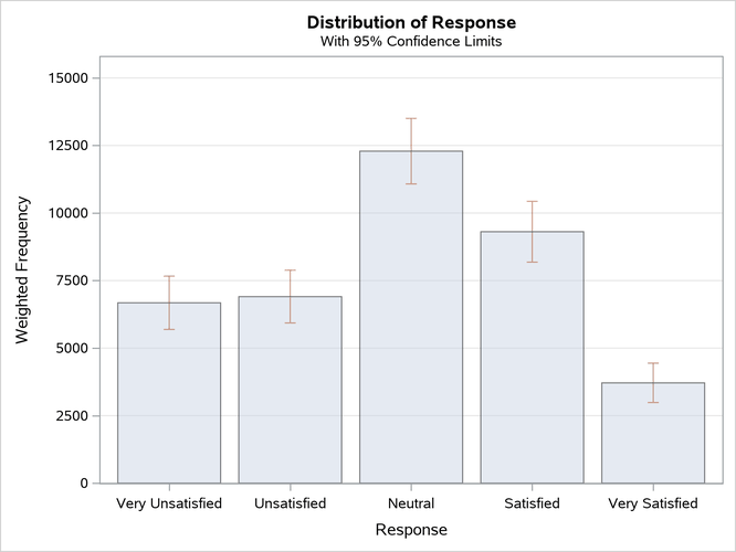
Figure 5 shows the chi-square goodness-of-fit test for the distribution of Response. The null hypothesis for this test is equal proportions for the levels of the one-way frequency table. (To test a null hypothesis of proportions that are not equal, you can use the TESTP= option to specify null hypothesis proportions.)
The CHISQ option produces the Rao-Scott design-adjusted chi-square test, which takes into account the sample design and provides inferences for the study population. To compute the Rao-Scott chi-square statistic, PROC SURVEYFREQ computes the Pearson chi-square statistic by using the weighted frequencies and adjusts this value by using a design correction. The procedure also provides an F approximation. For the table of Response, the F value is 30.0972 and the corresponding p-value is <0.0001, which indicates rejection of the null hypothesis of equal proportions.
Figure 5: Chi-Square Goodness-of-Fit Test for Response
| Rao-Scott Chi-Square Test | |
|---|---|
| Pearson Chi-Square | 251.8105 |
| Design Correction | 2.0916 |
| Rao-Scott Chi-Square | 120.3889 |
| DF | 4 |
| Pr > ChiSq | <.0001 |
| F Value | 30.0972 |
| Num DF | 4 |
| Den DF | 1456 |
| Pr > F | <.0001 |
| Sample Size = 1850 | |
The following PROC SURVEYFREQ statements request a two-way crosstabulation of SchoolType by Response:
title 'Student Information System Survey';
ods graphics on;
proc surveyfreq data=SIS_Survey nosummary;
   tables  SchoolType * Response /
      plots=wtfreqplot(type=dot scale=percent groupby=row);
   strata  State NewUser;
   cluster School;
   weight  SamplingWeight;
run;
ods graphics off;
The STRATA, CLUSTER, and WEIGHT statements do not change from the one-way analysis because the sample design and the input data set are the same. The PROC SURVEYFREQ statements request a different table but specify the same sample design information.
The ODS GRAPHICS ON statement enables ODS Graphics. The PLOTS= option in the TABLES statement requests a plot of SchoolType by Response, and the TYPE=DOT plot-option specifies a dot plot instead of the default bar chart. The SCALE=PERCENT plot-option requests a plot of percentages instead of totals. The GROUPBY=ROW plot-option groups the graph cells by the row variable (SchoolType).
Figure 6 shows the two-way crosstabulation table for SchoolType by Response. The first variable in the two-way table request, SchoolType, is the row variable, and the second variable, Response, is the column variable. Two-way tables display all column variable levels for each row variable level. This two-way table lists all levels of the column variable Response for each level of the row variable SchoolType, 'Middle School' and 'High School'. SchoolType='Total' shows the distribution of Response overall for both types of schools. Response='Total' provides totals over all levels of response for each type of school and overall. To suppress these totals, you can specify the NOTOTAL option.
Figure 6: Two-Way Table of SchoolType by Response
| Student Information System Survey |
| Table of SchoolType by Response | ||||||
|---|---|---|---|---|---|---|
| SchoolType | Response | Frequency | Weighted Frequency |
Std Err of Wgt Freq |
Percent | Std Err of Percent |
| Middle School | Very Unsatisfied | 116 | 2496 | 351.43834 | 6.4155 | 0.9030 |
| Unsatisfied | 109 | 2389 | 321.97957 | 6.1427 | 0.8283 | |
| Neutral | 234 | 4856 | 504.20553 | 12.4847 | 1.2953 | |
| Satisfied | 197 | 4064 | 443.71188 | 10.4467 | 1.1417 | |
| Very Satisfied | 94 | 1952 | 302.17144 | 5.0193 | 0.7758 | |
| Total | 750 | 15758 | 1000 | 40.5089 | 2.5691 | |
| High School | Very Unsatisfied | 188 | 4183 | 431.30589 | 10.7521 | 1.1076 |
| Unsatisfied | 217 | 4518 | 446.31768 | 11.6137 | 1.1439 | |
| Neutral | 347 | 7434 | 574.17175 | 19.1119 | 1.4726 | |
| Satisfied | 258 | 5245 | 498.03221 | 13.4845 | 1.2823 | |
| Very Satisfied | 90 | 1762 | 255.67158 | 4.5290 | 0.6579 | |
| Total | 1100 | 23142 | 1003 | 59.4911 | 2.5691 | |
| Total | Very Unsatisfied | 304 | 6678 | 501.61039 | 17.1676 | 1.2872 |
| Unsatisfied | 326 | 6907 | 495.94101 | 17.7564 | 1.2712 | |
| Neutral | 581 | 12291 | 617.20147 | 31.5965 | 1.5795 | |
| Satisfied | 455 | 9309 | 572.27868 | 23.9311 | 1.4761 | |
| Very Satisfied | 184 | 3714 | 370.66577 | 9.5483 | 0.9523 | |
| Total | 1850 | 38900 | 129.85268 | 100.0000 | ||
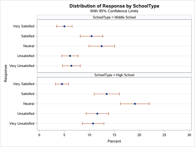
Figure 7 displays the weighted frequency dot plot that PROC SURVEYFREQ produces for the table of SchoolType and Response. The GROUPBY=ROW plot-option groups the graph cells by the row variable (SchoolType). If you do not specify GROUPBY=ROW, the procedure groups the graph cells by the column variable by default. You can plot percentages instead of weighted frequencies by specifying the SCALE=PERCENT plot-option. You can use other plot-options to change the orientation of the plot or to request a different two-way layout.
Figure 7: Dot Plot of Percentages for SchoolType by Response
The following PROC SURVEYFREQ statements request a two-way table of SchoolType by Response that displays row percentages and a chi-square test of association between the two variables:
title 'Student Information System Survey';
proc surveyfreq data=SIS_Survey nosummary;
   tables  SchoolType * Response / row nowt chisq;
   strata  State NewUser;
   cluster School;
   weight  SamplingWeight;
run;
The ROW option in the TABLES statement requests row percentages, which provide the distribution of Response within each level of the row variable SchoolType. The NOWT option suppresses display of the weighted frequencies and their standard errors. The CHISQ option requests a Rao-Scott chi-square test of association between SchoolType and Response.
Figure 8 displays the two-way table of SchoolType by Response. For middle schools, it is estimated that 25.79% of school personnel are satisfied with the student information system and 12.39% are very satisfied. For high schools, these estimates are 22.67% and 7.61%, respectively.
Figure 9 displays the chi-square test results. The Rao-Scott chi-square statistic is 9.04, and the corresponding F value is 2.26 with a p-value of 0.0605. This indicates an association between school type (middle school or high school) and satisfaction with the student information system at the 10% significance level.
Figure 8: Two-Way Table with Row Percentages
| Student Information System Survey |
| Table of SchoolType by Response | ||||||
|---|---|---|---|---|---|---|
| SchoolType | Response | Frequency | Percent | Std Err of Percent |
Row Percent |
Std Err of Row Percent |
| Middle School | Very Unsatisfied | 116 | 6.4155 | 0.9030 | 15.8373 | 1.9920 |
| Unsatisfied | 109 | 6.1427 | 0.8283 | 15.1638 | 1.8140 | |
| Neutral | 234 | 12.4847 | 1.2953 | 30.8196 | 2.5173 | |
| Satisfied | 197 | 10.4467 | 1.1417 | 25.7886 | 2.2947 | |
| Very Satisfied | 94 | 5.0193 | 0.7758 | 12.3907 | 1.7449 | |
| Total | 750 | 40.5089 | 2.5691 | 100.0000 | ||
| High School | Very Unsatisfied | 188 | 10.7521 | 1.1076 | 18.0735 | 1.6881 |
| Unsatisfied | 217 | 11.6137 | 1.1439 | 19.5218 | 1.7280 | |
| Neutral | 347 | 19.1119 | 1.4726 | 32.1255 | 2.0490 | |
| Satisfied | 258 | 13.4845 | 1.2823 | 22.6663 | 1.9240 | |
| Very Satisfied | 90 | 4.5290 | 0.6579 | 7.6128 | 1.0557 | |
| Total | 1100 | 59.4911 | 2.5691 | 100.0000 | ||
| Total | Very Unsatisfied | 304 | 17.1676 | 1.2872 | ||
| Unsatisfied | 326 | 17.7564 | 1.2712 | |||
| Neutral | 581 | 31.5965 | 1.5795 | |||
| Satisfied | 455 | 23.9311 | 1.4761 | |||
| Very Satisfied | 184 | 9.5483 | 0.9523 | |||
| Total | 1850 | 100.0000 | ||||
Figure 9: Chi-Square Test of No Association
| Rao-Scott Chi-Square Test | |
|---|---|
| Pearson Chi-Square | 18.7829 |
| Design Correction | 2.0766 |
| Rao-Scott Chi-Square | 9.0450 |
| DF | 4 |
| Pr > ChiSq | 0.0600 |
| F Value | 2.2613 |
| Num DF | 4 |
| Den DF | 1456 |
| Pr > F | 0.0605 |
| Sample Size = 1850 | |