ODS Graphics Template Modification

The following steps show how to create displays that have varying numbers of graphs:

proc glm noprint data=sashelp.baseball;
   class div;
   model logsalary = div CrHome;
   output out=pvals p=p;
quit;

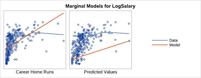
%marginal(independents=CrHome, dependent=LogSalary, predicted=p,
          panel=1 3, gopts=designheight=250px)

proc glm noprint data=sashelp.baseball;
   class div;
   model logsalary = div CrHome CrRuns;
   output out=pvals p=p;
quit;

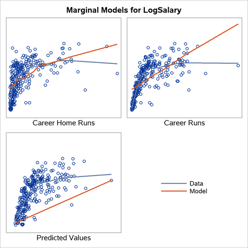
%marginal(independents=CrHome CrRuns, dependent=LogSalary, predicted=p)

%let vars = nHits nHome nRuns CrHits CrHome CrRuns CrRbi;

proc glm noprint data=sashelp.baseball;
   class div;
   model logsalary = div &vars;
   output out=pvals p=p;
quit;

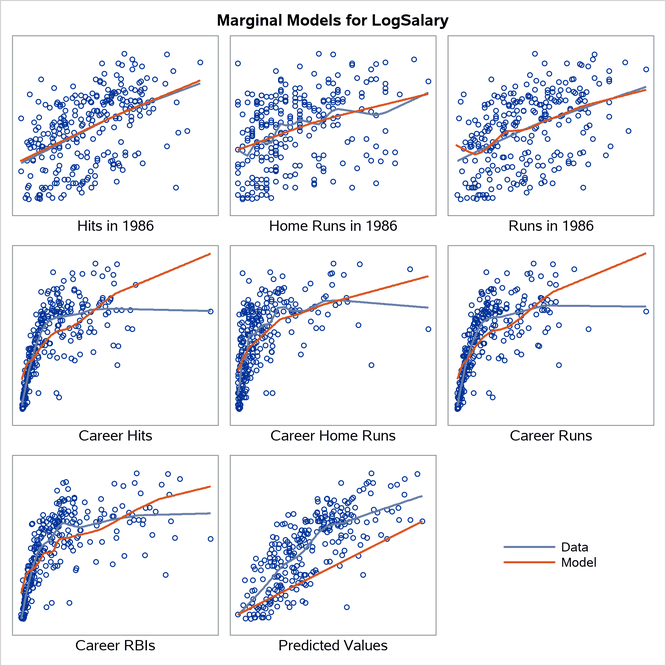
%marginal(independents=&vars, dependent=LogSalary, predicted=p)

proc glm noprint data=sashelp.baseball;
   class div;
   model logsalary = div CrAtBat CrHits CrHome;
   output out=pvals p=p;
quit;

%marginal(independents=CrAtBat CrHits CrHome,
          dependent=LogSalary, predicted=p, panel=1)

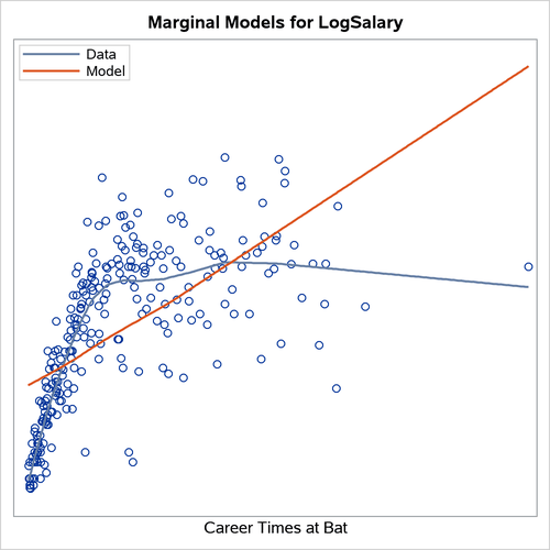
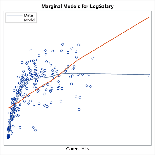
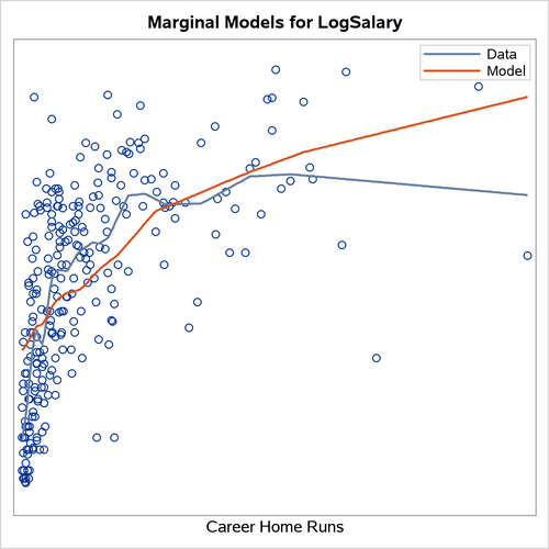
In the first model, the PANEL=1 3 and GOPTS=DESIGNHEIGHT=250PX options create a display. The results are displayed in Output 25.7.2. In the second model, the default display for three graphs is . The results are displayed in Output 25.7.3. In the third model, the default display for eight graphs is . The results are displayed in Output 25.7.4. In the fourth model, the PANEL=1 option creates single graphs. The results are displayed in Output 25.7.5.

When you display graphs in panels, the legend occupies one of the cells. When you produce single graphs, the legend appears inside each graph.

Output 25.7.2: 1 by 3 Display

Output 25.7.3: 2 by 2 Display

Output 25.7.4: 3 by 3 Display

Output 25.7.5: Single-Graph Display