The VARIOGRAM Procedure
Example 131.5 A Box Plot of the Square Root Difference Cloud
(View the complete code for this example.)
The Gaussian form selected for the semivariogram in the section Getting Started: VARIOGRAM Procedure is based on consideration of the plots of the sample semivariogram. For the coal thickness data, the Gaussian form appears to be a reasonable choice.
However, it can often happen that a plot of the sample variogram shows so much scatter that no particular form is evident. The cause of this scatter can be one or more outliers in the pairwise differences of the measured quantities.
A method of identifying potential outliers is discussed in Cressie (1993, section 2.2.2). This example illustrates how to use the OUTPAIR= data set from PROC VARIOGRAM to produce a square root difference cloud, which is useful in detecting outliers.
For the SRF  , the square root difference cloud for a particular direction
  is given by

for a given lag distance h. In the actual computation, all pairs  of points
  ,
,  within a distance tolerance around h and an angle tolerance around the direction
  are used. This generates a number of point pairs for each lag class h. The spread of these values gives an indication of outliers.
Following the example in the section Getting Started: VARIOGRAM Procedure, this example uses a basic LAGDISTANCE=7, with a distance tolerance of 3.5, and a direction of N–S, with an angle tolerance ATOL=30 .
.
First, use PROC VARIOGRAM to produce an OUTPAIR= data set. Then use a DATA step to subset this data by choosing pairs within 30 of N–S. In addition, compute lag class and square root difference variables, as the following statements show:
title 'Square Root Difference Cloud Example';

proc variogram data=sashelp.thick outp=outp noprint;
   compute novariogram;
   coordinates xc=East yc=North;
   var Thick;
run;
data sqroot;
   set outp;
   /*- Include only points +/- 30 degrees of N-S -------*/
   where abs(cos) < 0.5;
   /*- Unit lag of 7, distance tolerance of 3.5 --------*/
   lag_class=int(distance/7 + 0.5000001);
   sqr_diff=sqrt(abs(v1-v2));
run;
proc sort data=sqroot;
   by lag_class;
run;
Next, summarize the results by using the MEANS procedure:
proc means data=sqroot noprint n mean std;
   var sqr_diff;
   by lag_class;
   output out=msqrt n=n mean=mean std=std;
run;
title2 'Summary of Results';
proc print data=msqrt;
   id lag_class;
   var n mean std;
run;
The preceding statements produce Output 131.5.1.
Output 131.5.1: Summary of Results
| Square Root Difference Cloud Example |
| Summary of Results |
| lag_class | n | mean | std |
|---|---|---|---|
| 0 | 5 | 0.47300 | 0.14263 |
| 1 | 31 | 0.77338 | 0.41467 |
| 2 | 51 | 1.17052 | 0.47800 |
| 3 | 58 | 1.52287 | 0.51454 |
| 4 | 65 | 1.68625 | 0.58465 |
| 5 | 65 | 1.66963 | 0.68582 |
| 6 | 80 | 1.79693 | 0.62929 |
| 7 | 88 | 1.73334 | 0.73191 |
| 8 | 83 | 1.75528 | 0.68767 |
| 9 | 108 | 1.72901 | 0.58274 |
| 10 | 80 | 1.48268 | 0.48695 |
| 11 | 84 | 1.19242 | 0.47037 |
| 12 | 68 | 0.89765 | 0.42510 |
| 13 | 38 | 0.84223 | 0.44249 |
| 14 | 7 | 1.05653 | 0.42548 |
| 15 | 3 | 1.35076 | 0.11472 |
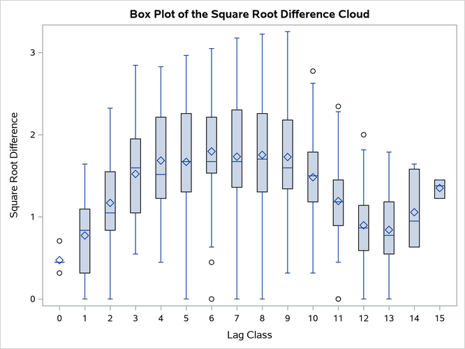
Finally, present the results in a box plot by using the SGPLOT procedure. The box plot facilitates the detection of outliers. The statements are as follows:
proc sgplot data=sqroot;
   xaxis label = "Lag Class";
   yaxis label = "Square Root Difference";
   title "Box Plot of the Square Root Difference Cloud";
   vbox sqr_diff / category=lag_class;
run;
Output 131.5.2 suggests that outliers, if any, do not appear to be adversely affecting the empirical semivariogram in the N–S direction for the coal seam thickness data. The conclusion from Output 131.5.2 is consistent with our previous semivariogram analysis of the same data set in the section Getting Started: VARIOGRAM Procedure. The effect of the isolated outliers in lag classes 6 and 10–12 in Output 131.5.2 is demonstrated as the divergence between the classical and robust empirical semivariance estimates in the higher distances in Figure 7. The difference in these estimates comes from the definition of the robust semivariance estimator  (see the section Theoretical and Computational Details of the Semivariogram), which imposes a smoothing effect on the outlier influence.
Output 131.5.2: Box Plot of the Square Root Difference Cloud