The GLIMMIX Procedure
Example 52.20 Comparison of Predictive Margins in Multicenter Study
(View the complete code for this example.)
It is often useful to compare the average response rates of treatment groups in clinical trials. This example shows how to compute predictive margins to account for covariates distributions in such a comparison.
Consider a multicenter study that investigates the performance of two treatments. In this study, ten treatment centers are randomly selected for inclusion. At each center, patients are randomly assigned to treatment A or treatment B. One of the study goals is to compare the response rates of the treatments.
The data set multicenter, created in the following DATA step, has five variables. The variable trt identifies the two treatments. The variable marker takes a value of 1 if the patient is biomarker-positive, and 0 if the patient is biomarker-negative. The response variable is 1 if the patient responds to the treatment, and 0 if the patient does not.
data multicenter;
   input center trt$ age marker response @@;
   datalines;
 1 A  15  0  0     1 A  28  0  0
 1 A  60  0  1     1 A  68  1  1
 1 A  23  1  0     1 A  33  1  1
 1 A  30  1  0     1 A  73  1  1
 1 A  15  1  0     1 A  34  1  0
 1 A  15  1  0     1 A  68  1  1
 1 B  53  0  1     1 B  62  0  1
 1 B  15  0  0     1 B  28  1  0
 1 B  27  1  0     1 B  45  1  0
 1 B  56  1  1     1 B  24  1  0
 1 B  42  1  0     1 B  61  1  0
 1 B  15  1  0     1 B  67  1  1
 2 A  28  0  1     2 A  43  0  1
 2 A  52  0  1     2 A  49  1  1
 2 A  59  1  1     2 A  32  1  1
 2 A  50  1  1     2 A  41  1  1
 2 A  21  1  0     2 A  62  1  1
 2 A  77  1  1     2 A  70  1  1
 2 B  79  0  1     2 B  49  0  1
 2 B  73  0  1     2 B  73  1  1
 2 B  78  1  1     2 B  61  1  1
 2 B  78  1  1     2 B  54  1  1
 2 B  51  1  1     2 B  50  1  1
 2 B  17  1  0     2 B  15  1  0
 3 A  20  0  0     3 A  18  0  1
 3 A  32  0  1     3 A  55  1  1
 3 A  51  1  1     3 A  58  1  1
 3 A  36  1  1     3 A  15  1  0
 3 A  21  1  0     3 A  24  1  1
 3 A  40  1  1     3 A  28  1  0
 3 B  54  0  1     3 B  64  0  1
 3 B  15  0  0     3 B  15  1  0
 3 B  76  1  1     3 B  39  1  1
 3 B  48  1  0     3 B  34  1  0
 3 B  17  1  0     3 B  37  1  0
 3 B  35  1  0     3 B  30  1  1
 4 A  74  0  1     4 A  78  0  1
 4 A  15  1  0     4 A  41  1  1
 4 A  25  1  0     4 A  31  1  0
 4 A  22  1  0     4 A  15  1  0
 4 B  77  0  1     4 B  33  0  0
 4 B  21  1  0     4 B  15  1  0
 4 B  70  1  1     4 B  54  1  0
 4 B  15  1  0     4 B  15  1  0
 5 A  21  0  1     5 A  72  0  1
 5 A  28  1  1     5 A  58  1  1
 5 A  39  1  1     5 A  41  1  1
 5 A  35  1  0     5 A  59  1  1
 5 B  73  0  1     5 B  15  0  0
 5 B  46  1  1     5 B  59  1  1
 5 B  20  1  0     5 B  66  1  1
 5 B  24  1  0     5 B  15  1  0
 6 A  25  0  0     6 A  15  0  0
 6 A  63  1  1     6 A  15  1  0
 6 A  61  1  1     6 A  73  1  1
 6 A  35  1  0     6 A  76  1  1
 6 B  76  0  1     6 B  15  0  0
 6 B  15  1  0     6 B  15  1  0
 6 B  15  1  0     6 B  47  1  0
 6 B  77  1  1     6 B  17  1  0
 7 A  27  0  0     7 A  18  0  0
 7 A  18  0  1     7 A  62  1  1
 7 A  30  1  0     7 A  25  1  0
 7 A  40  1  0     7 A  18  1  0
 7 A  16  1  0     7 A  17  1  0
 7 A  43  1  1     7 A  24  1  0
 7 B  64  0  1     7 B  29  0  0
 7 B  23  0  0     7 B  20  1  0
 7 B  36  1  0     7 B  46  1  0
 7 B  19  1  0     7 B  41  1  0
 7 B  23  1  0     7 B  40  1  1
 7 B  37  1  1     7 B  22  1  0
 8 A  51  0  1     8 A  85  0  1
 8 A  16  1  1     8 A  37  1  1
 8 A  28  1  0     8 A  24  1  0
 8 A  25  1  0     8 A  17  1  0
 8 B  54  0  1     8 B  21  0  1
 8 B  23  1  0     8 B  20  1  0
 8 B  19  1  0     8 B  18  1  0
 8 B  21  1  0     8 B  22  1  0
 9 A  22  0  0     9 A  23  0  0
 9 A  33  1  0     9 A  68  1  1
 9 A  42  1  1     9 A  51  1  1
 9 A  16  1  0     9 A  52  1  1
 9 B  77  0  1     9 B  16  0  0
 9 B  42  1  0     9 B  59  1  1
 9 B  28  1  0     9 B  33  1  0
 9 B  31  1  0     9 B  20  1  0
10 A  30  0  1    10 A  24  0  1
10 A  18  1  0    10 A  16  1  0
10 A  27  1  1    10 A  29  1  1
10 A  40  1  1    10 A  64  1  1
10 B  32  0  1    10 B  25  0  0
10 B  19  1  0    10 B  22  1  0
10 B  23  1  0    10 B  38  1  0
10 B  18  1  1    10 B  23  1  0
;
For patient j at center i, the logistic regression model is

where  is the probability that patient j at center i has responded to the treatment;
  is the random effect for center i; I is the indicator function;
  and
and  are the effects of treatments A and B, respectively;
  and
and  are the effects of a positive biomarker and a negative biomarker, respectively; and finally,
  ,
,  ,
,  , and
, and  are the interaction effects of
 trt and marker.
Given this model, the predictive margin for treatment A is

where  is the number of patients at treatment center i,
  is the number of patients in the study, and
  is the inverse logistic link function. The predictive margin for treatment A is the average predicted response rate if all patients receive treatment A.
Similarly, the predictive margin for treatment B is

This is the average predicted response rate if all patients receive treatment B.
The following statements fit the multicenter data to the logistic regression model:
proc glimmix data=multicenter;
   class center trt marker;
   model response = trt|marker age/s dist=binary link=logit;
   random  intercept/ subject=center;
   margins trt/ diff;
   margins trt*marker/ sliceby=marker slicediff;
run;
The first MARGINS statement requests predictive margins for the two treatment groups. The DIFF option compares average treatment response rates that control for the age and biomarker distributions.
Figure 141 shows the predictive margins for treatment A and treatment B.
Figure 141: Treatment Predictive Margins
| trt Margins | |||||
|---|---|---|---|---|---|
| trt | Estimate | Standard Error | DF | t Value | Pr > |t| |
| A | 0.4481 | 0.05349 | 178 | 8.38 | <.0001 |
| B | 0.6296 | 0.04276 | 178 | 14.72 | <.0001 |
Figure 142 shows the test of the difference between the two treatment predictive margins.
Figure 142: Difference of Treatment Margins
| Differences of trt Margins | ||||||
|---|---|---|---|---|---|---|
| trt | _trt | Estimate | Standard Error | DF | t Value | Pr > |t| |
| A | B | -0.1815 | 0.04689 | 178 | -3.87 | 0.0002 |
The degrees of freedom in Figure 141 and Figure 142 are the same as those in the "Type III Tests of Fixed Effect" table (not shown). Based on the p-value, you would conclude that at the 0.05 level the average response rates of treatment A and treatment B are significantly different.
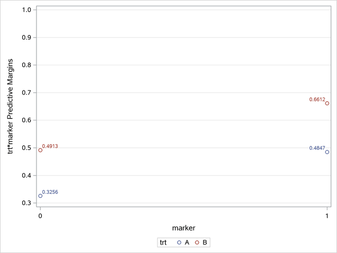
The second MARGINS statement requests predictive margins for the trt*marker interaction. The results are shown in Figure 143.
Figure 143: trt*marker Predictive Margins
| trt*marker Margins | ||||||
|---|---|---|---|---|---|---|
| trt | marker | Estimate | Standard Error | DF | t Value | Pr > |t| |
| A | 0 | 0.3256 | 0.08589 | 178 | 3.79 | 0.0002 |
| A | 1 | 0.4847 | 0.05322 | 178 | 9.11 | <.0001 |
| B | 0 | 0.4913 | 0.08996 | 178 | 5.46 | <.0001 |
| B | 1 | 0.6612 | 0.04152 | 178 | 15.93 | <.0001 |
The four predictive margins in Figure 143 are plotted in Output 52.20.1.
Output 52.20.1: Predictive Margins for trt*marker
To test the significance of the treatment difference within each biomarker group, you can use the SLICEBY option, which slices the trt*marker interaction by the marker effect. The SLICEDIFF option then compares the sliced predictive margins for the biomarker-positive group and the biomarker-negative group separately.
Figure 144 shows the test of the treatment margin difference for the biomarker-negative group.
Figure 144: Treatment Margins Difference in Biomarker-Negative Group
| Differences of trt*marker Margins Sliced by marker | |||||||
|---|---|---|---|---|---|---|---|
| Slice | trt | _trt | Estimate | Standard Error | DF | t Value | Pr > |t| |
| marker 0 | A | B | -0.1657 | 0.1101 | 178 | -1.50 | 0.1343 |
Figure 145 shows the test of the treatment margin difference for the biomarker-positive group.
Figure 145: Treatment Margins Difference in Biomarker-Positive Group
| Differences of trt*marker Margins Sliced by marker | |||||||
|---|---|---|---|---|---|---|---|
| Slice | trt | _trt | Estimate | Standard Error | DF | t Value | Pr > |t| |
| marker 1 | A | B | -0.1765 | 0.05013 | 178 | -3.52 | 0.0005 |
Figure 145 shows that the average response rates are significantly different between treatment A and treatment B in the biomarker-positive group (p-value of 0.0005) whereas the average response rates are not significantly different in the biomark-negative group (p-value of 0.13, Figure 144).