The LOGISTIC Procedure
Getting Started: LOGISTIC Procedure
(View the complete code for this example.)
The LOGISTIC procedure is similar in use to the other regression procedures in the SAS System. To demonstrate the similarity, suppose the response variable y is binary or ordinal, and x1 and x2 are two explanatory variables of interest. To fit a logistic regression model, you can specify a MODEL statement similar to that used in the REG procedure. For example:
proc logistic;
   model y=x1 x2;
run;
The response variable y can be either character or numeric. PROC LOGISTIC enumerates the total number of response categories and orders the response levels according to the response variable option ORDER= in the MODEL statement.
You can also input binary response data that are grouped. In the following statements, n represents the number of trials and r represents the number of events:
proc logistic;
   model r/n=x1 x2;
run;
The following example illustrates the use of PROC LOGISTIC. The data, taken from Cox and Snell (1989, pp. 10–11), consist of the number, r, of ingots not ready for rolling, out of n tested, for a number of combinations of heating time and soaking time.
data ingots;
   input Heat Soak r n @@;
   datalines;
7 1.0 0 10  14 1.0 0 31  27 1.0 1 56  51 1.0 3 13
7 1.7 0 17  14 1.7 0 43  27 1.7 4 44  51 1.7 0  1
7 2.2 0  7  14 2.2 2 33  27 2.2 0 21  51 2.2 0  1
7 2.8 0 12  14 2.8 0 31  27 2.8 1 22  51 4.0 0  1
7 4.0 0  9  14 4.0 0 19  27 4.0 1 16
;
The following invocation of PROC LOGISTIC fits the binary logit model to the grouped data. The continuous covariates Heat and Soak are specified as predictors, and the bar notation ("|") includes their interaction, Heat*Soak. The ODDSRATIO statement produces odds ratios in the presence of interactions, and a graphical display of the requested odds ratios is produced when ODS Graphics is enabled.
ods graphics on;
proc logistic data=ingots;
   model r/n = Heat | Soak;
   oddsratio Heat / at(Soak=1 2 3 4);
run;
The results of this analysis are shown in the following figures. PROC LOGISTIC first lists background information in Figure 1 about the fitting of the model. Included are the name of the input data set, the response variable(s) used, the number of observations used, and the link function used.
Figure 1: Binary Logit Model
| Model Information | |
|---|---|
| Data Set | WORK.INGOTS |
| Response Variable (Events) | r |
| Response Variable (Trials) | n |
| Model | binary logit |
| Optimization Technique | Fisher's scoring |
| Number of Observations Read | 19 |
|---|---|
| Number of Observations Used | 19 |
| Sum of Frequencies Read | 387 |
| Sum of Frequencies Used | 387 |
The "Response Profile" table (Figure 2) lists the response categories (which are Event and Nonevent when grouped data are input), their ordered values, and their total frequencies for the given data.
Figure 2: Response Profile for Grouped Data with Events/Trials Syntax
| Response Profile | ||
|---|---|---|
| Ordered Value |
Binary Outcome | Total Frequency |
| 1 | Event | 12 |
| 2 | Nonevent | 375 |
| Model Convergence Status |
|---|
| Convergence criterion (GCONV=1E-8) satisfied. |
The "Model Fit Statistics" table (Figure 3) contains Akaike’s information criterion (AIC), the Schwarz criterion (SC), and the negative of twice the log likelihood (–2 Log L) for the intercept-only model and the fitted model. AIC and SC can be used to compare different models, and the ones with smaller values are preferred. Results of the likelihood ratio test and the efficient score test for testing the joint significance of the explanatory variables (Soak, Heat, and their interaction) are included in the "Testing Global Null Hypothesis: BETA=0" table (Figure 3); the small p-values reject the hypothesis that all slope parameters are equal to zero.
Figure 3: Fit Statistics and Hypothesis Tests
| Model Fit Statistics | |||
|---|---|---|---|
| Criterion | Intercept Only | Intercept and Covariates | |
| Log Likelihood | Full Log Likelihood | ||
| AIC | 108.988 | 103.222 | 35.957 |
| SC | 112.947 | 119.056 | 51.791 |
| -2 Log L | 106.988 | 95.222 | 27.957 |
| Testing Global Null Hypothesis: BETA=0 | |||
|---|---|---|---|
| Test | Chi-Square | DF | Pr > ChiSq |
| Likelihood Ratio | 11.7663 | 3 | 0.0082 |
| Score | 16.5417 | 3 | 0.0009 |
| Wald | 13.4588 | 3 | 0.0037 |
The "Analysis of Maximum Likelihood Estimates" table in Figure 4 lists the parameter estimates, their standard errors, and the results of the Wald test for individual parameters. Note that the Heat*Soak parameter is not significantly different from zero (p=0.727), nor is the Soak variable (p=0.6916).
Figure 4: Parameter Estimates
| Analysis of Maximum Likelihood Estimates | |||||
|---|---|---|---|---|---|
| Parameter | DF | Estimate | Standard Error |
Wald Chi-Square |
Pr > ChiSq |
| Intercept | 1 | -5.9901 | 1.6666 | 12.9182 | 0.0003 |
| Heat | 1 | 0.0963 | 0.0471 | 4.1895 | 0.0407 |
| Soak | 1 | 0.2996 | 0.7551 | 0.1574 | 0.6916 |
| Heat*Soak | 1 | -0.00884 | 0.0253 | 0.1219 | 0.7270 |
The "Association of Predicted Probabilities and Observed Responses" table (Figure 5) contains four measures of association for assessing the predictive ability of a model. They are based on the number of pairs of observations with different response values, the number of concordant pairs, and the number of discordant pairs, which are also displayed. Formulas for these statistics are given in the section Rank Correlation of Observed Responses and Predicted Probabilities.
Figure 5: Association Table
| Association of Predicted Probabilities and Observed Responses |
|||
|---|---|---|---|
| Percent Concordant | 73.2 | Somers' D | 0.541 |
| Percent Discordant | 19.1 | Gamma | 0.586 |
| Percent Tied | 7.6 | Tau-a | 0.033 |
| Pairs | 4500 | c | 0.771 |
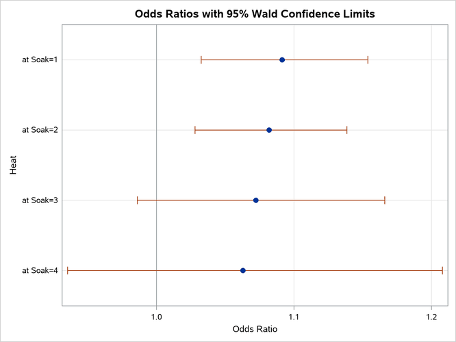
The ODDSRATIO statement produces the "Odds Ratio Estimates and Wald Confidence Intervals" table (Figure 6), and a graphical display of these estimates is shown in Figure 7. The differences between the odds ratios are small compared to the variability shown by their confidence intervals, which confirms the previous conclusion that the Heat*Soak parameter is not significantly different from zero.
Figure 6: Odds Ratios of Heat at Several Values of Soak
| Odds Ratio Estimates and Wald Confidence Intervals | |||
|---|---|---|---|
| Odds Ratio | Estimate | 95% Confidence Limits | |
| Heat at Soak=1 | 1.091 | 1.032 | 1.154 |
| Heat at Soak=2 | 1.082 | 1.028 | 1.139 |
| Heat at Soak=3 | 1.072 | 0.986 | 1.166 |
| Heat at Soak=4 | 1.063 | 0.935 | 1.208 |
Figure 7: Plot of Odds Ratios of Heat at Several Values of Soak
Because the Heat*Soak interaction is nonsignificant, the following statements fit a main-effects model:
proc logistic data=ingots;
   model r/n = Heat Soak;
run;
The results of this analysis are shown in the following figures. The model information and response profiles are the same as those in Figure 1 and Figure 2 for the saturated model. The "Model Fit Statistics" table in Figure 8 shows that the AIC and SC for the main-effects model are smaller than for the saturated model, indicating that the main-effects model might be the preferred model. As in the preceding model, the "Testing Global Null Hypothesis: BETA=0" table indicates that the parameters are significantly different from zero.
Figure 8: Fit Statistics and Hypothesis Tests
| Model Fit Statistics | |||
|---|---|---|---|
| Criterion | Intercept Only | Intercept and Covariates | |
| Log Likelihood | Full Log Likelihood | ||
| AIC | 108.988 | 101.346 | 34.080 |
| SC | 112.947 | 113.221 | 45.956 |
| -2 Log L | 106.988 | 95.346 | 28.080 |
| Testing Global Null Hypothesis: BETA=0 | |||
|---|---|---|---|
| Test | Chi-Square | DF | Pr > ChiSq |
| Likelihood Ratio | 11.6428 | 2 | 0.0030 |
| Score | 15.1091 | 2 | 0.0005 |
| Wald | 13.0315 | 2 | 0.0015 |
The "Analysis of Maximum Likelihood Estimates" table in Figure 9 again shows that the Soak parameter is not significantly different from zero (p=0.8639). The odds ratio for each effect parameter, estimated by exponentiating the corresponding parameter estimate, is shown in the "Odds Ratios Estimates" table (Figure 9), along with 95% Wald confidence intervals. The confidence interval for the Soak parameter contains the value 1, which also indicates that this effect is not significant.
Figure 9: Parameter Estimates and Odds Ratios
| Analysis of Maximum Likelihood Estimates | |||||
|---|---|---|---|---|---|
| Parameter | DF | Estimate | Standard Error |
Wald Chi-Square |
Pr > ChiSq |
| Intercept | 1 | -5.5592 | 1.1197 | 24.6503 | <.0001 |
| Heat | 1 | 0.0820 | 0.0237 | 11.9454 | 0.0005 |
| Soak | 1 | 0.0568 | 0.3312 | 0.0294 | 0.8639 |
| Odds Ratio Estimates | |||
|---|---|---|---|
| Effect | Point Estimate | 95% Wald Confidence Limits |
|
| Heat | 1.085 | 1.036 | 1.137 |
| Soak | 1.058 | 0.553 | 2.026 |
| Association of Predicted Probabilities and Observed Responses |
|||
|---|---|---|---|
| Percent Concordant | 73.0 | Somers' D | 0.537 |
| Percent Discordant | 19.3 | Gamma | 0.581 |
| Percent Tied | 7.6 | Tau-a | 0.032 |
| Pairs | 4500 | c | 0.769 |
Using these parameter estimates, you can calculate the estimated logit of  as
as

For example, if Heat=7 and Soak=1, then logit . Using this logit estimate, you can calculate
  as follows:

This gives the predicted probability of the event (ingot not ready for rolling) for Heat=7 and Soak=1. Note that PROC LOGISTIC can calculate these statistics for you; use the OUTPUT statement with the PREDICTED= option, or use the SCORE statement.
To illustrate the use of an alternative form of input data, the following program creates the ingots data set with the new variables NotReady and Freq instead of n and r. The variable NotReady represents the response of individual units; it has a value of 1 for units not ready for rolling (event) and a value of 0 for units ready for rolling (nonevent). The variable Freq represents the frequency of occurrence of each combination of Heat, Soak, and NotReady. Note that, compared to the previous data set, NotReady=1 implies Freq=r, and NotReady=0 implies Freq=n–r.
data ingots;
   input Heat Soak NotReady Freq @@;
   datalines;
7 1.0 0 10  14 1.0 0 31  14 4.0 0 19  27 2.2 0 21  51 1.0 1  3
7 1.7 0 17  14 1.7 0 43  27 1.0 1  1  27 2.8 1  1  51 1.0 0 10
7 2.2 0  7  14 2.2 1  2  27 1.0 0 55  27 2.8 0 21  51 1.7 0  1
7 2.8 0 12  14 2.2 0 31  27 1.7 1  4  27 4.0 1  1  51 2.2 0  1
7 4.0 0  9  14 2.8 0 31  27 1.7 0 40  27 4.0 0 15  51 4.0 0  1
;
The following statements invoke PROC LOGISTIC to fit the main-effects model by using the alternative form of the input data set:
proc logistic data=ingots;
   model NotReady(event='1') = Heat Soak;
   freq Freq;
run;
Results of this analysis are the same as the preceding grouped main-effects analysis. The displayed output for the two runs are identical except for the background information of the model fit and the "Response Profile" table shown in Figure 10.
Figure 10: Response Profile with Single-Trial Syntax
| Response Profile | ||
|---|---|---|
| Ordered Value |
NotReady | Total Frequency |
| 1 | 0 | 375 |
| 2 | 1 | 12 |
| Probability modeled is NotReady=1. |
By default, Ordered Values are assigned to the sorted response values in ascending order, and PROC LOGISTIC models the probability of the response level that corresponds to the Ordered Value 1. There are several methods to change these defaults; the preceding statements specify the response variable option EVENT= to model the probability of NotReady=1 as displayed in Figure 10. For more information, see the section Response Level Ordering.