Statistical Graphics Using ODS

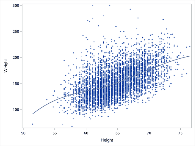
You can use PROC SGPLOT and the REG statement along with the DEGREE=3 option to fit a cubic polynomial function to your data. A cubic polynomial is smooth and has little freedom to follow nonlinear trends in the data. The model is

The following step creates the plot in Output 24.6.1:

proc sgplot data=sashelp.heart noautolegend;
   reg y=weight x=height / markerattrs=(size=3px) degree=3;
run;

Output 24.6.1: Cubic Polynomial Fit Plot

You can use the PBSPLINE statement to fit penalized B-splines (Eilers and Marx 1996). Penalized B-splines draw a smooth curve through a scatter plot by using an automatic selection of the smoothing parameter. The following step creates the plot in Output 24.6.2:

ods graphics on / antialiasmax=6000;
proc sgplot data=sashelp.heart noautolegend;
   pbspline y=weight x=height / markerattrs=(size=3px);
run;

Output 24.6.2: Penalized B-Spline Fit Plot

The resulting fit function is smooth and nonlinear. You do not need to know anything about the shape of the scatter plot. The PBSPLINE statement automatically finds a smooth fit while trying to guard against overfitting. It is not possible to write a simple equation for the model. For more information about how penalized B-splines work, see Chapter 126, The TRANSREG Procedure.

Note: Antialiasing smooths the elements of a graph. The ANTIALIASMAX=6000 option enables antialiasing through 6,000 elements. By default, antialiasing is disabled after 4,000 elements.

You can use the LOESS statement to find a loess fit function (Cleveland, Devlin, and Grosse 1988). Loess is a locally weighted scatter plot smoothing. The following step creates the plot in Output 24.6.3:

ods graphics on / loessmaxobs=6000;
proc sgplot data=sashelp.heart noautolegend;
   loess y=weight x=height / markerattrs=(size=3px);
run;

Output 24.6.3: Loess Fit Plot

The loess fit is not a spline fit, but loess is similar to penalized B-splines in that it automatically tries to find a smooth fit while trying to guard against overfitting. It is not possible to write a simple equation for the model. For more information about loess, see Chapter 78, The LOESS Procedure.

Note: Loess becomes computationally expensive with larger data sets. The LOESSOBSMAX=6000 option enables loess fits through 6,000 observations. By default, loess fits are disabled after 5,000 observations.

You can use the PBSPLINE statement along with the option SMOOTH=0 to fit B-splines (De Boor 1978), which are equivalent to piecewise-polynomial splines. You specify SMOOTH=0 to disable all automatic smoothing. You specify the number of knots in the NKNOTS= option.^[13] You use fewer knots to create smoother plots and more knots to enable greater curvature. The following step creates the plot in Output 24.6.4:

proc sgplot data=sashelp.heart noautolegend;
   pbspline y=weight x=height / smooth=0 nknots=5 markerattrs=(size=3px);
run;

Output 24.6.4: B-Spline Fit Plot

The resulting fit function is equivalent to those that you can obtain by using SPLINE (spline transformation), PSPLINE (polynomial-spline basis), or BSPLINE (B-spline basis) in the MODEL statement in PROC TRANSREG. Of all the functions shown in Output 24.6.2 through Output 24.6.4, the B-spline fit in Output 24.6.4 is most influenced by the extreme X values. The polynomial-spline model is

The values through are the knots, which fall in the range of x. When is negative, ; otherwise, . The expression is called a truncated power function. Each knot term changes the cubic part of the polynomial as x advances beyond each knot.

For an introduction to piecewise-polynomial splines, see Smith (1979). For more information about how splines work, see Chapter 126, The TRANSREG Procedure.