Statistical Graphics Using ODS

Multiple Fit Functions Using PROC SGPLOT

The next set of steps shows the same methods that were shown in the section Single Fit Function Using PROC SGPLOT but this time using different data and a group variable.

Polynomial Fit Functions

You can use the REG statement with the DEGREE= and GROUP= options to fit multiple polynomial functions. The following step creates the plot in Output 24.6.9:

proc sgplot data=sashelp.gas;
   reg y=nox x=eqratio / degree=3 group=fuel markerattrs=(size=3px) name='a';
   keylegend 'a' / location=inside position=topright across=1;
run;

Output 24.6.9: Grouped Cubic Polynomial Fit Plot

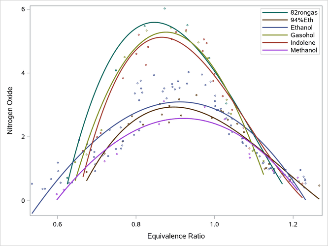
The plot in Output 24.6.9 contains six cubic polynomial functions, each independent of the others. Each function has the form

y Subscript i Baseline equals beta Subscript i Baseline 0 Baseline plus beta Subscript i Baseline 1 Baseline x plus beta Subscript i Baseline 2 Baseline x squared plus beta Subscript i Baseline 3 Baseline x cubed plus epsilon

If is a binary indicator variable (i = 1 to 6) such that , is 1 for 82rongas and 0 for all other fuels, is 1 for 94%Eth and 0 for all other fuels, and so on, then

y equals sigma-summation Underscript i equals 1 Overscript 6 Endscripts c Subscript i Baseline left-bracket beta Subscript i Baseline 0 Baseline plus beta Subscript i Baseline 1 Baseline x plus beta Subscript i Baseline 2 Baseline x squared plus beta Subscript i Baseline 3 Baseline x cubed right-bracket plus epsilon

Penalized B-Spline Fit Functions

You can use the PBSPLINE statement with the GROUP= option to fit multiple penalized B-splines. The following step creates the plot in Output 24.6.10:

proc sgplot data=sashelp.gas;
   pbspline y=nox x=eqratio / group=fuel markerattrs=(size=3px) name='a';
   keylegend 'a' / location=inside position=topright across=1;
run;

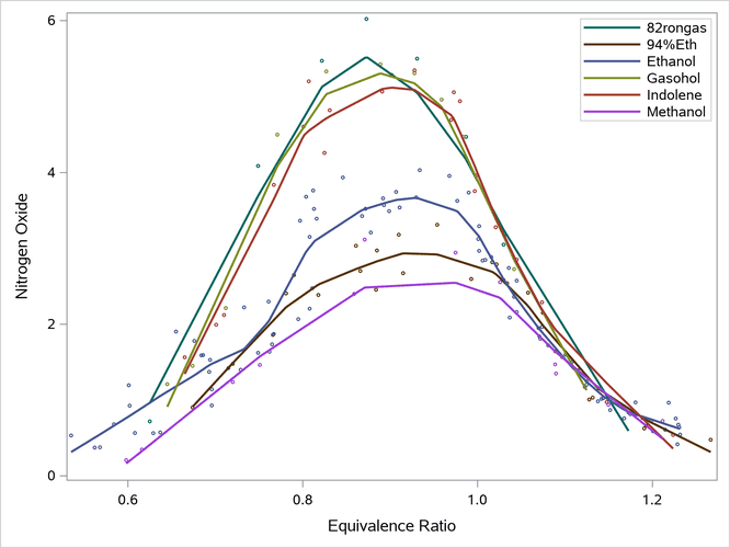
Output 24.6.10: Grouped Penalized B-Spline Fit Plot

The penalized B-spline fit functions are less smooth than the polynomials.

Loess Fit Functions

You can use the LOESS statement with the GROUP= option to fit multiple loess curves. The following step creates the plot in Output 24.6.11:

proc sgplot data=sashelp.gas;
   loess y=nox x=eqratio / group=fuel markerattrs=(size=3px) name='a';
   keylegend 'a' / location=inside position=topright across=1;
run;

Output 24.6.11: Grouped Loess Fit Plot

The loess spline fit functions are less smooth than the polynomials.

B-Spline Fit Functions

You can use the PBSPLINE statement, the SMOOTH=0 and NKNOTS= options, and the GROUP= option to fit multiple B-spline functions. The following step creates the plot in Output 24.6.12:

proc sgplot data=sashelp.gas;
   pbspline y=nox x=eqratio / group=fuel smooth=0 nknots=5
                              markerattrs=(size=3px) name='a';
   keylegend 'a' / location=inside position=topright across=1;
run;

Output 24.6.12: Grouped B-Spline Fit Plot

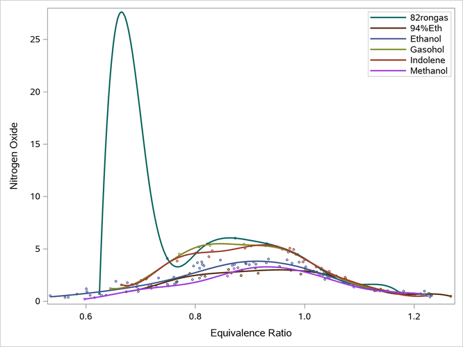
The polynomial-spline function is unsatisfactory for the 82rongas function. This is because there is a large gap between the first two points. The function connects the dots between the first several points, and it is free to deviate from the data between points. This is a frequent concern with splines. Having fixed knots that apply to all functions, no matter how sparse they are, is problematic. In contrast, penalized B-splines and loess automatically smooth that section of that function. The polynomial functions do not have enough parameters to enable that level of nonlinearity.

Last updated: December 09, 2022