The PSMATCH Procedure
Example 101.8 Matching with Precomputed Propensity Scores
(View the complete code for this example.)
The PSMATCH procedure provides the capability for fitting a binary logistic regression model that is used to compute propensity scores for matching. However, there might be situations in which you have already computed the propensity scores—for example, by using other procedures in SAS/STAT software that perform logistic regression. This example illustrates optimal matching with precomputed propensity scores that are provided in the input data set for PROC PSMATCH.
The data for this example are observations on patients in a nonrandomized clinical trial. The trial and the Drugs data set that contains the patient information are described in the section Getting Started: PSMATCH Procedure.
The following statements use the LOGISTIC procedure to derive propensity scores:
ods select none;
proc logistic data=drugs;
   class Drug Gender;
   model Drug(Event='Drug_X')= Gender Age BMI / link=cloglog;
   output out=drug1 p=pscore;
run;
ods select all;
The LINK=CLOGLOG option fits the complementary log-log model and derives propensity scores that are used in the PSMATCH procedure. The option is used just to demonstrate that, other than the logit link that is provided in the PSMATCH procedure, you can use a different model to derive propensity scores and then input these propensity scores in the PSMATCH procedure.
The output data set Drug1 is constructed from the data set Drugs and contains the PScore variable for propensity scores.
Output 101.8.1 lists the first 10 observations.
Output 101.8.1: Data Set with Propensity Scores
| Obs | PatientID | Drug | Gender | Age | BMI | pscore |
|---|---|---|---|---|---|---|
| 1 | 284 | Drug_X | Male | 29 | 22.02 | 0.35498 |
| 2 | 201 | Drug_A | Male | 45 | 26.68 | 0.21794 |
| 3 | 147 | Drug_A | Male | 42 | 21.84 | 0.12261 |
| 4 | 307 | Drug_X | Male | 38 | 22.71 | 0.19821 |
| 5 | 433 | Drug_A | Male | 31 | 22.76 | 0.34298 |
| 6 | 435 | Drug_A | Male | 43 | 26.86 | 0.26261 |
| 7 | 159 | Drug_A | Female | 45 | 25.47 | 0.15077 |
| 8 | 368 | Drug_A | Female | 49 | 24.28 | 0.08713 |
| 9 | 286 | Drug_A | Male | 31 | 23.31 | 0.37211 |
| 10 | 163 | Drug_X | Female | 39 | 25.34 | 0.24005 |
The following statements request optimal matching to match patients in the treatment group to patients in the control group:
ods graphics on;
proc psmatch data=Drug1 region=cs;
   class Drug Gender;
   psdata treatvar=Drug(Treated='Drug_X') ps=pscore;
   match method=optimal(k=1) exact=Gender distance=lps caliper=0.5
         weight=none;
   assess lps var=(Gender Age BMI);
   output out(obs=match)=OutEx8 lps=_Lps matchid=_MatchID;
run;
The PSMODEL statement is not used in this example because the propensity scores are provided in Drug1. Instead, the PSDATA statement is used to identify the binary treatment variable and the propensity score variable in Drug1. The CLASS statement specifies the classification variables. The PS= option specifies pscore as the propensity score variable. The TREATVAR=DRUG option specifies Drug as the binary treatment indicator variable, and TREATED='Drug_X' identifies Drug_X as the treated group.
The PSMATCH procedure matches only those observations whose propensity scores lie in the support region that you specify with the REGION= option. Here the REGION=CS option requests that only those observations whose propensity scores (or equivalently, logits of propensity scores) lie in the common support region be used for matching. The common support region is the largest interval that contains propensity scores (or equivalently, logits of propensity scores) for both treated and control observations. By default, the region is extended by 0.25 times the pooled estimate of the common standard deviation of the logits of the propensity scores.
The MATCH statement specifies the criteria for matching. The DISTANCE=LPS option (which is the default) requests that the logit of the propensity score be used in computing differences between pairs of observations. The METHOD=OPTIMAL(K=1) option (which is the default) requests optimal matching of one control unit to each unit in the treated group in order to minimize the total within-pair difference. The EXACT=GENDER option requests that the treated unit and its matched control unit have the same value of the Gender variable. The CALIPER=0.5 option requests that a match be made only if the difference in the logits of the propensity scores for pairs of individuals is less than or equal to 0.5 times the pooled estimate of the common standard deviation of the logits of the propensity scores.
The "Data Information" table in Output 101.8.2 displays the numbers of observations in the treated and control groups, the lower and upper limits for the propensity scores of observations in the support region, and the numbers of observations in the treated and control groups that fall within the support region. Of the 373 observations in the control group, 352 fall within the support region.
Output 101.8.2: Data Information
| Data Information | |
|---|---|
| Data Set | WORK.DRUG1 |
| Output Data Set | WORK.OUTEX8 |
| Treatment Variable | Drug |
| Treated Group | Drug_X |
| All Obs (Treated) | 113 |
| All Obs (Control) | 373 |
| Support Region | Extended Common Support |
| Lower PS Support | 0.060563 |
| Upper PS Support | 0.698199 |
| Support Region Obs (Treated) | 113 |
| Support Region Obs (Control) | 352 |
The "Propensity Score Information" table in Output 101.8.3 displays summary statistics by treatment group for all observations, for observations in the support region, and for matched observations.
Output 101.8.3: Propensity Score Information
| Propensity Score Information | |||||||||||
|---|---|---|---|---|---|---|---|---|---|---|---|
| Observations | Treated (Drug = Drug_X) | Control (Drug = Drug_A) | Treated - Control |
||||||||
| N | Mean | Standard Deviation |
Minimum | Maximum | N | Mean | Standard Deviation |
Minimum | Maximum | Mean Difference |
|
| All | 113 | 0.3040 | 0.1287 | 0.0715 | 0.6594 | 373 | 0.2089 | 0.1255 | 0.0295 | 0.7135 | 0.0952 |
| Region | 113 | 0.3040 | 0.1287 | 0.0715 | 0.6594 | 352 | 0.2146 | 0.1177 | 0.0606 | 0.6519 | 0.0894 |
| Matched | 113 | 0.3040 | 0.1287 | 0.0715 | 0.6594 | 113 | 0.2984 | 0.1215 | 0.0723 | 0.6519 | 0.0056 |
The "Matching Information" table in Output 101.8.4 displays the matching criteria, the number of matched sets, the numbers of matched observations in the treated and control groups, and the total absolute difference in the logits of the propensity scores for all matches.
Output 101.8.4: Matching Information
| Matching Information | |
|---|---|
| Distance Metric | Logit of Propensity Score |
| Method | Optimal Fixed Ratio Matching |
| Control/Treated Ratio | 1 |
| Caliper (Logit PS) | 0.356051 |
| Matched Sets | 113 |
| Matched Obs (Treated) | 113 |
| Matched Obs (Control) | 113 |
| Total Absolute Difference | 3.616259 |
The ASSESS statement produces tables and plots that summarize differences in the distributions of the specified variables between treated and control groups for all observations, for observations in the support region, and for matched observations. As requested by the LPS and VAR= options, the variables that are listed in the table are the logit of the propensity score and the variables Gender, Age, and BMI. The WEIGHT=NONE option suppresses the display of differences for the weighted matched observations. When one control unit is matched to each treated unit, the weights are all 1 for matched treated and control units, so the results for weighted matched observations and matched observations are identical.
The "Standardized Mean Differences" table displays standardized mean differences in the variables between the treated and control groups. For a binary classification variable (Gender), the difference is in the proportion of the first ordered level (Female).
Output 101.8.5: Standardized Mean Differences
| Standardized Mean Differences (Treated - Control) | ||||||
|---|---|---|---|---|---|---|
| Variable | Observations | Mean Difference |
Standard Deviation |
Standardized Difference |
Percent Reduction |
Variance Ratio |
| Logit Prop Score | All | 0.58239 | 0.712102 | 0.81785 | 0.7177 | |
| Region | 0.51613 | 0.72480 | 11.38 | 0.9052 | ||
| Matched | 0.02268 | 0.03184 | 96.11 | 1.0929 | ||
| Age | All | -4.09509 | 6.079104 | -0.67363 | 0.7076 | |
| Region | -3.58515 | -0.58975 | 12.45 | 0.7928 | ||
| Matched | 0.11504 | 0.01892 | 97.19 | 1.0143 | ||
| BMI | All | 0.73930 | 1.923178 | 0.38441 | 0.8854 | |
| Region | 0.65089 | 0.33845 | 11.96 | 0.9394 | ||
| Matched | 0.14619 | 0.07602 | 80.23 | 1.3509 | ||
| Gender | All | -0.02482 | 0.496925 | -0.04994 | 0.9892 | |
| Region | -0.01808 | -0.03638 | 27.16 | 0.9916 | ||
| Matched | 0.00000 | 0.00000 | 100.00 | 1.0000 | ||
| Standard deviation of All observations used to compute standardized differences | ||||||
The standardized mean differences are significantly reduced in the matched observations, and the largest of these differences is 0.076 in absolute value, which is less than the recommended upper limit of 0.25. The treated-to-control variance ratios between the two groups are between 1 and 1.3509 for all variables in the matched observations, which is within the recommended range of 0.5 to 2. Because both EXACT=GENDER and METHOD=OPTIMAL are specified in the MATCH statement, the standardized mean difference for Gender is 0 in the matched observations.
The PSMATCH procedure displays a standardized mean differences plot, as shown in Output 101.8.6, for the variables that are specified in the ASSESS statement.
Output 101.8.6: Standardized Mean Differences Plot
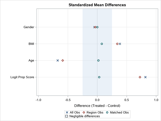
The "Standardized Mean Differences Plot" displays the standardized mean differences that are listed in the "Standardized Mean Differences" table in Output 101.8.5. All differences for the matched observations are within the recommended limits of –0.25 and 0.25, which are indicated by the shaded area.
Because matching results in good balance for the variables in this example, the matched observations can be saved in an output data set for use in a subsequent outcome analysis.
In situations where you are not satisfied with the variable balance, you can do one or more of the following to improve the balance: you can select another set of variables to fit the propensity score model, you can modify the matching criteria, or you can choose another matching method.
The OUT(OBS=MATCH)=OutEx8 option in the OUTPUT statement creates an output data set, OutEx8, that contains the matched observations. The following statements list the observations in the first five matched sets, as shown in Output 101.8.7:
proc sort data=OutEx8 out=OutEx8a;
   by _MatchID;
run;

proc print data=OutEx8a(obs=10);
   var PatientID Drug Gender Age BMI pscore _LPS _MatchWgt_ _MatchID;
run;
Output 101.8.7: Output Data Set With Optimal Matches
| Obs | PatientID | Drug | Gender | Age | BMI | pscore | _Lps | _MATCHWGT_ | _MatchID |
|---|---|---|---|---|---|---|---|---|---|
| 1 | 213 | Drug_A | Female | 49 | 23.24 | 0.07234 | -2.55123 | 1 | 1 |
| 2 | 89 | Drug_X | Female | 44 | 20.75 | 0.07152 | -2.56356 | 1 | 1 |
| 3 | 245 | Drug_A | Female | 52 | 25.32 | 0.08090 | -2.43015 | 1 | 2 |
| 4 | 323 | Drug_X | Female | 46 | 22.22 | 0.07822 | -2.46677 | 1 | 2 |
| 5 | 429 | Drug_A | Male | 49 | 24.00 | 0.09865 | -2.21228 | 1 | 3 |
| 6 | 217 | Drug_X | Male | 49 | 23.96 | 0.09796 | -2.22013 | 1 | 3 |
| 7 | 234 | Drug_X | Female | 41 | 21.11 | 0.09887 | -2.20987 | 1 | 4 |
| 8 | 66 | Drug_A | Female | 48 | 24.53 | 0.09927 | -2.20531 | 1 | 4 |
| 9 | 183 | Drug_A | Female | 45 | 23.62 | 0.10931 | -2.09786 | 1 | 5 |
| 10 | 320 | Drug_X | Female | 46 | 24.17 | 0.11056 | -2.08507 | 1 | 5 |
By default, the output data set includes the variable _PS_ (which provides the propensity score) and the variable _MATCHWGT_ (which provides matched observation weights). The weight for each treated unit is 1. Because K=1 is specified in the METHOD=OPTIMAL option in the MATCH statement, one control unit is matched to each treated unit, so the weight for each matched control unit is also 1. The LPS=_LPS option creates a variable named _LPS (which provides the logit of the propensity score) and the MATCHID=_MatchID option creates a variable named _MatchID (which identifies the matched sets of observations).
After the responses for the trial are observed, they can be added to the data set OutEx8 as the starting point for an outcome analysis. Assuming that no other confounding variables are associated with both the response variable and the treatment group indicator Drug, you can estimate the treatment effect from the matched observations by performing an outcome analysis that you would have used to estimate the treatment effect if the original data set had resulted from a randomized trial.