The CAUSALGRAPH Procedure
Example 37.7 Applying an Adjustment Set to Estimate a Causal Effect from Data
(View the complete code for this example.)
This example illustrates how you can use the CAUSALGRAPH procedure to estimate the magnitude of a causal effect that has a valid causal interpretation. To compute such an estimate from a data set, you can use the following general approach:
Carefully consider the data generating process, and create a list of causal assumptions that accurately represents that process. Encode these assumptions in a graphical causal model. For more information about causal assumptions and graphical models, see the section Causal Graph Theory.
Use this graphical model to find a valid identification strategy, such as an adjustment set.
Use the identification results to construct an estimator, such as the stratification estimator.
In most practical situations, the true data generating process is not known exactly. In such situations, you must define a causal model that is assumed to represent the data generating process. To construct this causal model, you might rely on expert opinion, established scientific theory, prior experience, or any other source of substantive knowledge. This example uses simulated data, so that the data generating process is treated as known and the impact of identification and adjustment on causal effect estimation can be illustrated. For more information about identification strategies and adjustment sets, see the section Identification by Adjustment.
A causal model that relates an individual’s serum urate to the risk of cardiovascular disease is shown in Figure 10. This model is derived from a larger model that was developed by Thornley et al. (2013). See Example 37.3 for a summary of the variables in the figure. The treatment and outcome variables are shaded in the model. For this example, the variable Nutrition corresponds to a latent construct and thus is not measured or observed. It is also assumed that the variable PreviousHDL is not measured.
Figure 10: Causal Model of the Effect of Serum Urate on Risk of Cardiovascular Disease
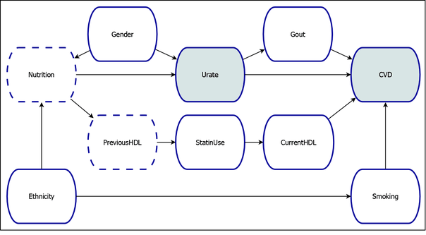
The following DATA step creates a simulated data set that is consistent with the model in Figure 10. Thus, it also defines the true data generating process.
data CVDdata;
   drop ii Nutrition PreviousHDL;
   call streaminit(1000);
   array EthProb[6] _temporary_ (0.60, 0.18, 0.13, 0.05, 0.01, 0.03);
   array SmokeRates[6] _temporary_ (0.17, 0.10, 0.17, 0.07, 0.22, 0.15);
   array EthNut[6] _temporary_ (0.20, 0.18, 0.08, 0.03, 0.11, 0.04);
   do ii = 1 to 79000;
      Gender = rand("Bernoulli" , .5);
      Ethnicity = rand("Table" , of EthProb[*]);
      Smoking = rand("Bernoulli", SmokeRates[Ethnicity]);
      Nutrition = 0.5 - Gender + 10.0*rand("Normal", 0, EthNut[Ethnicity]);
      PreviousHDL = 55 + 4.0*Nutrition;
      if      PreviousHDL<40 then StatinUse = rand("Bernoulli", 0.90);
      else if PreviousHDL<60 then StatinUse = rand("Bernoulli", 0.65);
      else                        StatinUse = rand("Bernoulli", 0.05);
      CurrentHDL = 55 + rand("Normal",0.0,7) + StatinUse*rand("Normal",4.0,0.5);
      Urate = 6.0 + 0.4*Nutrition + 1.5*Gender;
      Gout = rand("Bernoulli", logistic(-8.0 + 0.90*Urate));
      CVD = rand("Bernoulli", logistic(-1.2 - 0.04*CurrentHDL + 0.2*Gout +
         0.65*Smoking + 0.1*Urate));
      output;
   end;
run;
The first 10 lines of the simulated data set are shown in Output 37.7.1.
Output 37.7.1: First 10 Lines of the Simulated Data Set
| Obs | Gender | Ethnicity | Smoking | StatinUse | CurrentHDL | Urate | Gout | CVD |
|---|---|---|---|---|---|---|---|---|
| 1 | Female | Hispanic | No | 0 | 45.9241 | 6.41547 | 1 | 0 |
| 2 | Male | Hispanic | No | 1 | 66.9528 | 7.43840 | 0 | 0 |
| 3 | Female | NativeAmer | No | 1 | 54.5367 | 6.42775 | 0 | 0 |
| 4 | Female | Hispanic | No | 1 | 67.7733 | 5.32636 | 0 | 0 |
| 5 | Female | WhiteNonHisp | No | 0 | 64.2067 | 6.67543 | 0 | 0 |
| 6 | Male | WhiteNonHisp | No | 1 | 53.0462 | 7.22069 | 1 | 0 |
| 7 | Female | AfricanAmer | Yes | 1 | 49.4850 | 5.15609 | 0 | 0 |
| 8 | Male | Hispanic | Yes | 0 | 57.8065 | 6.47476 | 0 | 0 |
| 9 | Female | WhiteNonHisp | No | 0 | 57.7600 | 6.52005 | 0 | 1 |
| 10 | Male | AfricanAmer | No | 1 | 71.0460 | 7.30762 | 0 | 0 |
The following code uses the simulated data to create a table of summary statistics for the variable Urate:
proc means data=CVDdata;
   var Urate;
   ods output Summary=SampleMeansOutput;
run;
The summary statistics are shown in Output 37.7.2. You use the ODS OUTPUT statement to store the summary statistics for Urate in an output data set. You use this information later in the analysis to define the treatment and control levels for the causal effect of interest.
Output 37.7.2: Summary Statistics for Urate
| Analysis Variable : Urate | ||||
|---|---|---|---|---|
| N | Mean | Std Dev | Minimum | Maximum |
| 79000 | 6.7460150 | 0.8936312 | 3.0665877 | 10.3763707 |
In this example, the treatment or exposure variable Urate is continuous. Moreover, the effect of this variable on the mediator variable Gout and the outcome variable (CVD) is nonlinear. Because there are no natural treatment and control levels for Urate, you must somehow define the causal effect of interest. A common causal effect measure is the average treatment effect (ATE) or the expected risk difference, which is the difference in the expected potential outcome values between well-defined treatment and control conditions or levels. For more information about the definitions of causal effect measures in the potential outcome framework, see the section Causal Effects: Definitions, Assumptions, and Identification in Chapter 39, The CAUSALTRT Procedure.
In this example, you consider the causal effect of interest to be the expected risk difference in CVD that is associated with a change in Urate from a control condition to a treatment condition. Two possibilities for defining the control and treatment conditions are considered here. In this way, you can explore how the magnitude of the causal effect depends on the values of the treatment variable that are being considered.
First, you consider the causal effect of a unit change in Urate, centered around the population mean. Then, in the potential outcomes notation, the causal effect of interest is the expected risk difference

where  is the population mean of
 Urate. In this causal effect definition, the control condition is defined as a half unit below the population mean of Urate, and the treatment condition is defined as a half unit above the population mean of Urate.
Second, you consider the causal effect of a change of one standard deviation in Urate, also centered around the population mean. The causal effect is now defined as the expected risk difference

where  is the population standard deviation of
 Urate.
For demonstration purposes, the two population causal effects are computed by generating a large number of potential outcomes (1,000,000,000 replications) according to the true data generating process mentioned earlier. By this method, the population effect, UnitEff, is found to be 0.0076, and the standardized population effect, StdEff, is found to be 0.0068. These values are the target causal effects that you are estimating from the random sample. Now the most interesting questions are whether and how the CAUSALGRAPH procedure can help find a statistical strategy that provides accurate estimates of these target causal effects.
Given the causal model for the data, you can use the procedure to analyze the identifiability of the causal effect of Urate on CVD. The following code uses the procedure to list valid adjustment sets that can be used to identify this causal effect. For brevity, you can use the MAXSIZE=2 option to construct only those adjustment sets that have no more than two elements.
proc causalgraph maxsize=2;
   model "Thor12SimpleHDL"
      Ethnicity ==> Nutrition Smoking,
      Gender ==> Nutrition Urate,
      Gout ==> CVD,
      Nutrition ==> PreviousHDL Urate,
      CurrentHDL ==> CVD,
      PreviousHDL ==> StatinUse,
      Smoking ==> CVD,
      StatinUse ==> CurrentHDL,
      Urate ==> CVD Gout;
   identify Urate ==> CVD;
   unmeasured Nutrition PreviousHDL;
run;
In the MODEL statement, you specify the causal model to be analyzed. The quoted string in the statement labels the model. The remainder of the MODEL statement specifies all the variables and edges in the model. These variables and edges reflect the data generating process shown in Figure 10.
In the IDENTIFY statement, you specify that the causal effect of interest is the effect of Urate on CVD. In the UNMEASURED statement, you specify that the variables Nutrition and PreviousHDL are not measured or observed.
The list of adjustment sets that the procedure produces is shown in Output 37.7.3. Notice that the empty set does not appear in this list. This means that the marginal association between Urate and CVD cannot be used to estimate a causal effect that has a valid causal interpretation. Rather, you must use an alternative estimation strategy, such as estimation by adjustment that uses one of the adjustment sets in Output 37.7.3. As is shown later in this example, the failure to perform such an adjustment results in biased estimation of the causal effects.
Output 37.7.3: Possible Adjustment Sets for the Model in
| Covariate Adjustment Sets for Thor12SimpleHDL | ||||||||
|---|---|---|---|---|---|---|---|---|
| Causal Effect of Urate on CVD | ||||||||
| Size | Minimal | Covariates | ||||||
| CurrentHDL | Ethnicity | Gender | Gout | Smoking | StatinUse | |||
| 1 | 2 | Yes | * | * | ||||
| 2 | 2 | Yes | * | * | ||||
| 3 | 2 | Yes | * | * | ||||
| 4 | 2 | Yes | * | * | ||||
You can use any of the adjustments sets in Output 37.7.3 to obtain an estimate for the effect of Urate on CVD that has a valid causal interpretation. In particular, the set {Smoking, StatinUse} is a valid adjustment set. This set also has the useful property that both variables in the set are binary classification variables. Thus one possible way to estimate the causal effect is to stratify the analysis by the levels of these variables.
As mentioned earlier, two causal effects are being estimated. One is the unstandardized unit effect of Urate on CVD, denoted as UnitEff. The other is the standardized unit effect of Urate on CVD, denoted as StdEff. Both of these causal effects are defined in terms of the differences in expected CVD potential outcome values. These potential outcomes are evaluated at some Urate treatment and control levels that are defined in terms of population parameters. Because these population parameters and hence the treatment and control levels are not known, you need to estimate them from the sample. The following code computes two sets of sample values for the treatment and control levels of Urate from the table of summary statistics that you created earlier in this example. These computed values are stored in the data set ScoreData that you will use to estimate the two causal effects of interest.
data _null_;
   set SampleMeansOutput;
   call symputx("UrateMean",Urate_Mean);
   call symputx("UrateStd", Urate_StdDev);
   call symputx("UrateUnit1", Urate_Mean + 0.5);
   call symputx("UrateUnit0", Urate_Mean - 0.5);
   call symputx("UrateStd1", Urate_Mean + 0.5*Urate_StdDev);
   call symputx("UrateStd0", Urate_Mean - 0.5*Urate_StdDev);
run;

data ScoreData;
   set SampleMeansOutput;
   keep Urate Test;

   Test  = "UnitTreat  ";
   Urate = &UrateUnit1;
   output;

   Test  = "UnitControl";
   Urate = &UrateUnit0;
   output;

   Test  = "StdTreat   ";
   Urate = &UrateStd1;
   output;

   Test  = "StdControl ";
   Urate = &UrateStd0;
   output;
run;
Now, the following code performs logistic regression analyses that are stratified by levels of the two adjustment variables that are suggested by the results of PROC CAUSALGRAPH:
proc sort data=CVDdata;
   by Smoking StatinUse;
run;
proc logistic data=CVDdata noprint;
   by Smoking StatinUse;
   model CVD(event='1') = Urate;
   score data=ScoreData out=ProbStrat;
run;
The MODEL statement specifies the outcome variable CVD and the treatment variable Urate. The effect of Urate on CVD is estimated within each of the four strata separately. However, to estimate the aforementioned population causal effects of interest, you need to apply the logistic regression results to estimate the expected CVD values under the specific Urate treatment and control levels of interest. You can accomplish this by using the SCORE statement.
The SCORE statement estimates the probability of a CVD event (that is, the probability that CVD=1), which is the expected value of CVD, for each value of Urate that is specified in the data set ScoreData. In this example, these values of Urate correspond to the treatment and control levels for defining the causal effects of interest. Hence, the SCORE statement estimates the expected CVD values under the required treatment and control levels in each stratum. The OUT= option in the SCORE statement saves the expected CVD values in the data set ProbStrat. These expected CVD values are shown in the column P_1 in Output 37.7.4.
Output 37.7.4: Posterior Probabilities for Each Strata
| Obs | Smoking | StatinUse | Test | Urate | P_1 |
|---|---|---|---|---|---|
| 1 | 0 | 0 | UnitTreat | 7.24602 | 0.06929 |
| 2 | 0 | 0 | UnitControl | 6.24602 | 0.05994 |
| 3 | 0 | 0 | StdTreat | 7.19283 | 0.06876 |
| 4 | 0 | 0 | StdControl | 6.29920 | 0.06041 |
| 5 | 0 | 1 | UnitTreat | 7.24602 | 0.05829 |
| 6 | 0 | 1 | UnitControl | 6.24602 | 0.05489 |
| 7 | 0 | 1 | StdTreat | 7.19283 | 0.05811 |
| 8 | 0 | 1 | StdControl | 6.29920 | 0.05506 |
| 9 | 1 | 0 | UnitTreat | 7.24602 | 0.12451 |
| 10 | 1 | 0 | UnitControl | 6.24602 | 0.10476 |
| 11 | 1 | 0 | StdTreat | 7.19283 | 0.12338 |
| 12 | 1 | 0 | StdControl | 6.29920 | 0.10574 |
| 13 | 1 | 1 | UnitTreat | 7.24602 | 0.11226 |
| 14 | 1 | 1 | UnitControl | 6.24602 | 0.09918 |
| 15 | 1 | 1 | StdTreat | 7.19283 | 0.11153 |
| 16 | 1 | 1 | StdControl | 6.29920 | 0.09984 |
The two binary adjustment variables result in four strata for analysis. Within each stratum, you can compute the unstandardized unit effect by the difference in P_1 between UnitTreat and UnitControl, and you can compute the standardized effect by the difference in P_1 between StdTreat and StdControl. However, none of these effects within strata are the causal effect estimates themselves. The estimate of the causal effect UnitEff must be computed by using the weighted average of the difference in P_1 between UnitTreat and UnitControl in the strata, where the weights are the sample sizes of the strata. Similarly, the estimate of the causal effect StdEff must be computed by using the weighted average of the difference in P_1 between StdTreat and StdControl in the strata. These estimates of the causal effects are shown in the column Stratified Estimation in Output 37.7.6.
As discussed previously, if you attempt to estimate the effect of Urate on CVD by using the marginal association between the two variables (that is, no adjustment), confounding covariates bias the estimation results. Strictly for the purpose of demonstrating such a biased result, the following PROC LOGISTIC code performs a logistic regression that is not stratified by any covariate:
proc logistic data=CVDdata noprint;
   model CVD(event='1') = Urate;
   score data=ScoreData out=ProbNaive;
run;
Just as before, the SCORE statement in PROC LOGISTIC estimates the expected CVD values under the required Urate treatment and control levels. The corresponding estimates of the expected CVD values are shown in Output 37.7.5. As in the stratified estimation, the target causal effects are estimated by computing the related differences in P_1, except that in this case no weighted average is computed for the differences.
Output 37.7.5: Unadjusted Posterior Probabilities
| Obs | Test | Urate | P_1 |
|---|---|---|---|
| 1 | UnitTreat | 7.24602 | 0.073217 |
| 2 | UnitControl | 6.24602 | 0.064062 |
| 3 | StdTreat | 7.19283 | 0.072702 |
| 4 | StdControl | 6.29920 | 0.064521 |
Now, you have two sets of estimation results. One set of results is computed by using a stratified estimator that is based on an adjustment strategy. The other set of results is computed by using the naive marginal association between the treatment and outcome variables. The estimates of the causal effects UnitEff and StdEff that are computed using these two estimators are shown in Output 37.7.6. For comparison, the target true values of the causal effects are also shown.
Output 37.7.6: Causal Effect Estimation Summary
| Obs | Effect | True Effect | Stratified Estimation | Unadjusted Estimation |
|---|---|---|---|---|
| 1 | UnitEff | 0.007620 | 0.007766 | 0.009155 |
| 2 | StdEff | 0.006789 | 0.006940 | 0.008181 |
The estimates that are computed by using the stratified estimator very closely approximate the true values. This is expected, because the set {Smoking,StatinUse} is a valid adjustment set for the data generating process shown in Figure 10. However, the estimates that are computed by using the naive unadjusted logistic regression results do not agree with the true values. This is also expected, because the PROC CAUSALGRAPH analysis in Output 37.7.3 shows that the empty set is not a valid adjustment. Thus, this example demonstrates the usefulness of causal graph theory to identify causal effects in confounding situations. By devising a stratified estimator of the causal effects, this example also demonstrates how to implement a good statistical estimation strategy based on the identification results from PROC CAUSALGRAPH.