The CAUSALGRAPH Procedure
Getting Started: CAUSALGRAPH Procedure
(View the complete code for this example.)
This example demonstrates how you can use the CAUSALGRAPH procedure to determine which covariates in a causal model you must control in order to estimate a treatment effect that has a valid causal interpretation.
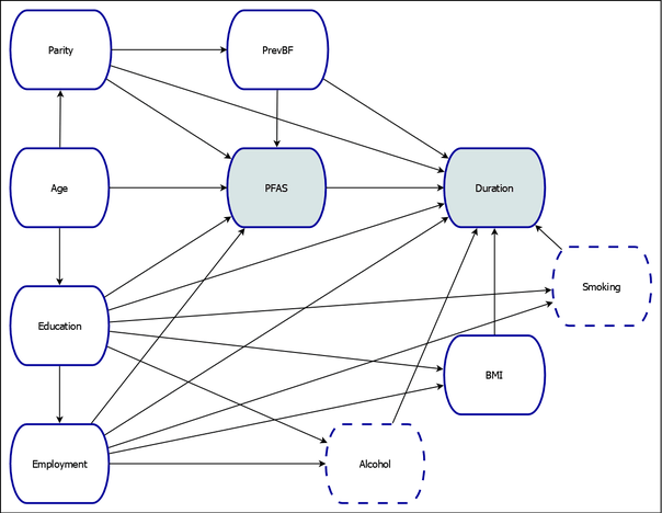
The causal model shown in Figure 1 has been adapted from Timmermann et al. (2017) and examines the relationship between maternal exposure to persistent perfluoroalkyl substances (PFAS) and breastfeeding duration (Duration) among residents of the Faroe Islands. The model includes the following variables:
PFAS: the treatment variableDuration: the outcome variableAge: age of the mother at the child’s birthEducation: indicator of whether the mother had any postprimary educationEmployment: a categorical variable that describes the employment condition of the mother (employed, unemployed, homemaker, and so on)Parity: indicator of whether this was the mother’s first childbirthAlcohol: indicator of whether the mother consumed alcohol during the pregnancySmoking: indicator of whether the mother smoked cigarettes during the pregnancyBMI: prepregnancy body mass index of the motherPrevBF: indicator of prior breastfeeding experience
The treatment (PFAS) and outcome (Duration) variables are shaded in Figure 1. For this example, it is assumed that the variables Alcohol and Smoking are not observed (for example, because the data are considered to be unreliable).
Figure 1: Causal Model of the Effect of Persistent Perfluoroalkyl Substances on Breastfeeding Duration
The statistical association between the variables PFAS and Duration that would be measured in an observational study reflects a combination of true causal association and additional spurious or noncausal association. In order to isolate the true causal association between PFAS and Duration, you must devise a strategy to eliminate the noncausal association. One way to do this is to find an adjustment set. You can use the CAUSALGRAPH procedure to construct all possible adjustment sets that can be used to identify the causal effect of PFAS on Duration, subject to the assumptions that are encoded in the causal model in Figure 1. If at least one such adjustment set exists, then it is possible to estimate the causal effect by using observational data. For more information about adjustment sets and identifying causal effects, see the section Identification by Adjustment.
The following statements invoke PROC CAUSALGRAPH to define and analyze the causal model and construct the adjustment sets:
proc causalgraph;
   model "Timm17TwoLatent"
      Age ==> Parity PFAS Education,
      Parity ==> PrevBF Duration PFAS,
      PrevBF ==> PFAS Duration,
      PFAS ==> Duration,
      Education ==> Duration Employment PFAS BMI Alcohol Smoking,
      Employment ==> Duration PFAS BMI Alcohol Smoking,
      BMI Alcohol Smoking ==> Duration;
   identify PFAS ==> Duration;
   unmeasured Alcohol Smoking;
run;
In an analysis that uses PROC CAUSALGRAPH, you must specify at least one causal model in a MODEL statement. You can also specify multiple models. Each MODEL statement must begin with a quoted string that provides a unique name for the model. This example labels the model as Timm17TwoLatent, a reference to its original publication. The remainder of the MODEL statement specifies the variables and their causal relationships (as indicated by directed edges). In this example, the MODEL statement encodes the model shown in Figure 1.
In the IDENTIFY statement, you specify the causal effect of interest. You can use this statement to specify one or more treatment variables and one or more outcome variables. The treatment and outcome variables are separated by a single right arrow, ==>. This example studies the causal effect of the variable PFAS on the variable Duration.
The UNMEASURED statement specifies variables that are not observed and thus cannot be included in any adjustment set. In this example, the variables Alcohol and Smoking are treated as unmeasured.
The output in Figure 2 summarizes the variables and edges in the causal model that is specified in the MODEL statement. You can use this information as a qualitative check of the model specification.
Figure 2: Input Summary Tables for the Causal Model in
| Variables in Model | ||
|---|---|---|
| N | Variables | |
| Measured | 8 | Age BMI Duration Education Employment Parity PFAS PrevBF |
| Unmeasured | 2 | Alcohol Smoking |
| Graphical Model Summary | ||||||
|---|---|---|---|---|---|---|
| Model | Nodes | Edges | Treatments | Outcomes | Measured | Unmeasured |
| Timm17TwoLatent | 10 | 23 | 1 | 1 | 8 | 2 |
In this example, the CAUSALGRAPH procedure uses the constructive backdoor criterion (METHOD=ADJUSTMENT; see Van der Zander, Liśkiewicz, and Textor 2014) to construct all valid adjustments. You can change the default criterion by specifying the METHOD= option in the PROC CAUSALGRAPH statement.
The adjustment sets are displayed in Figure 3. For the model in Figure 1, there are four valid adjustment sets. Each row of Figure 3 contains an adjustment set, and the variables in each set are indicated in the table by an asterisk. Assuming that the causal model is accurate, you can estimate the causal effect of PFAS on Duration by using any one of these adjustment sets.
Figure 3: Adjustment Sets for the Causal Model in
| Covariate Adjustment Sets for Timm17TwoLatent | ||||||||
|---|---|---|---|---|---|---|---|---|
| Causal Effect of PFAS on Duration | ||||||||
| Size | Minimal | Covariates | ||||||
| Age | BMI | Education | Employment | Parity | PrevBF | |||
| 1 | 4 | Yes | * | * | * | * | ||
| 2 | 5 | No | * | * | * | * | * | |
| 3 | 5 | No | * | * | * | * | * | |
| 4 | 6 | No | * | * | * | * | * | * |
The table also indicates the size of each set and whether or not the set is minimal. An adjustment set is minimal if no proper subset of the set is also a valid adjustment set. In this example, there is one minimal set that contains four covariates that you must adjust for in order to estimate the specified causal effect. You can use one of these covariate adjustment sets as input for an appropriate statistical procedure, such as PROC PSMATCH or PROC CAUSALTRT, to estimate the magnitude of the specified causal effect. For an illustration of how you can use an adjustment set to estimate a causal effect, see Example 37.7.
By default, PROC CAUSALGRAPH constructs every possible adjustment set for the specified causal effect. You can use the MAXLIST=, MAXSIZE=, and MINIMAL options in the PROC CAUSALGRAPH statement to refine the adjustment sets that are computed. You can modify the displayed output by using the LIST, NOLIST, NOPRINT, or PSUMMARY option in the PROC CAUSALGRAPH statement.