The LOGISTIC Procedure
Example 79.3 Ordinal Logistic Regression
(View the complete code for this example.)
Consider a study of the effects on taste of various cheese additives. Researchers tested four cheese additives and obtained 52 response ratings for each additive. Each response was measured on a scale of nine categories ranging from strong dislike (1) to excellent taste (9). The data, given in McCullagh and Nelder (1989, p. 175) in the form of a two-way frequency table of additive by rating, are saved in the data set Cheese by using the following program. The variable y contains the response rating. The variable Additive specifies the cheese additive (1, 2, 3, or 4). The variable freq gives the frequency with which each additive received each rating.
data Cheese;
   do Additive = 1 to 4;
      do y = 1 to 9;
         input freq @@;
         output;
      end;
   end;
   label y='Taste Rating';
   datalines;
0  0  1  7  8  8 19  8  1
6  9 12 11  7  6  1  0  0
1  1  6  8 23  7  5  1  0
0  0  0  1  3  7 14 16 11
;
The response variable y is ordinally scaled. A cumulative logit model is used to investigate the effects of the cheese additives on taste. The following statements invoke PROC LOGISTIC to fit this model with y as the response variable and three indicator variables as explanatory variables, with the fourth additive as the reference level. With this parameterization, each Additive parameter compares an additive to the fourth additive. The COVB option displays the estimated covariance matrix, and the NOODDSRATIO option suppresses the default odds ratio table. The ODDSRATIO statement computes odds ratios for all combinations of the Additive levels. The PLOTS option produces a graphical display of the odds ratios, and the EFFECTPLOT statement displays the predicted probabilities.
ods graphics on;
proc logistic data=Cheese plots(only)=oddsratio(range=clip);
   freq freq;
   class Additive (param=ref ref='4');
   model y=Additive / covb nooddsratio;
   oddsratio Additive;
   effectplot / polybar;
   title 'Multiple Response Cheese Tasting Experiment';
run;
The "Response Profile" table in Output 79.3.1 shows that the strong dislike (y=1) end of the rating scale is associated with lower Ordered Values in the "Response Profile" table; hence the probability of disliking the additives is modeled.
The score chi-square for testing the proportional odds assumption is 17.287, which is not significant with respect to a chi-square distribution with 21 degrees of freedom  . This indicates that the proportional odds assumption is reasonable. The positive value (1.6128) for the parameter estimate for
 Additive1 indicates a tendency toward the lower-numbered categories of the first cheese additive relative to the fourth. In other words, the fourth additive tastes better than the first additive. The second and third additives are both less favorable than the fourth additive. The relative magnitudes of these slope estimates imply the preference ordering: fourth, first, third, second.
Output 79.3.1: Proportional Odds Model Regression Analysis
| Multiple Response Cheese Tasting Experiment |
| Model Information | ||
|---|---|---|
| Data Set | WORK.CHEESE | |
| Response Variable | y | Taste Rating |
| Number of Response Levels | 9 | |
| Frequency Variable | freq | |
| Model | cumulative logit | |
| Optimization Technique | Fisher's scoring | |
| Number of Observations Read | 36 |
|---|---|
| Number of Observations Used | 28 |
| Sum of Frequencies Read | 208 |
| Sum of Frequencies Used | 208 |
| Response Profile | ||
|---|---|---|
| Ordered Value |
y | Total Frequency |
| 1 | 1 | 7 |
| 2 | 2 | 10 |
| 3 | 3 | 19 |
| 4 | 4 | 27 |
| 5 | 5 | 41 |
| 6 | 6 | 28 |
| 7 | 7 | 39 |
| 8 | 8 | 25 |
| 9 | 9 | 12 |
| Probabilities modeled are cumulated over the lower Ordered Values. |
| Note: | 8 observations having nonpositive frequencies or weights were excluded since they do not contribute to the analysis. |
| Class Level Information | ||||
|---|---|---|---|---|
| Class | Value | Design Variables | ||
| Additive | 1 | 1 | 0 | 0 |
| 2 | 0 | 1 | 0 | |
| 3 | 0 | 0 | 1 | |
| 4 | 0 | 0 | 0 | |
| Model Convergence Status |
|---|
| Convergence criterion (GCONV=1E-8) satisfied. |
| Score Test for the Proportional Odds Assumption |
||
|---|---|---|
| Chi-Square | DF | Pr > ChiSq |
| 17.2866 | 21 | 0.6936 |
| Model Fit Statistics | ||
|---|---|---|
| Criterion | Intercept Only | Intercept and Covariates |
| AIC | 875.802 | 733.348 |
| SC | 902.502 | 770.061 |
| -2 Log L | 859.802 | 711.348 |
| Testing Global Null Hypothesis: BETA=0 | |||
|---|---|---|---|
| Test | Chi-Square | DF | Pr > ChiSq |
| Likelihood Ratio | 148.4539 | 3 | <.0001 |
| Score | 111.2670 | 3 | <.0001 |
| Wald | 115.1504 | 3 | <.0001 |
| Type 3 Analysis of Effects | |||
|---|---|---|---|
| Effect | DF | Wald Chi-Square |
Pr > ChiSq |
| Additive | 3 | 115.1504 | <.0001 |
| Analysis of Maximum Likelihood Estimates | ||||||
|---|---|---|---|---|---|---|
| Parameter | DF | Estimate | Standard Error |
Wald Chi-Square |
Pr > ChiSq | |
| Intercept | 1 | 1 | -7.0801 | 0.5624 | 158.4851 | <.0001 |
| Intercept | 2 | 1 | -6.0249 | 0.4755 | 160.5500 | <.0001 |
| Intercept | 3 | 1 | -4.9254 | 0.4272 | 132.9484 | <.0001 |
| Intercept | 4 | 1 | -3.8568 | 0.3902 | 97.7087 | <.0001 |
| Intercept | 5 | 1 | -2.5205 | 0.3431 | 53.9704 | <.0001 |
| Intercept | 6 | 1 | -1.5685 | 0.3086 | 25.8374 | <.0001 |
| Intercept | 7 | 1 | -0.0669 | 0.2658 | 0.0633 | 0.8013 |
| Intercept | 8 | 1 | 1.4930 | 0.3310 | 20.3439 | <.0001 |
| Additive | 1 | 1 | 1.6128 | 0.3778 | 18.2265 | <.0001 |
| Additive | 2 | 1 | 4.9645 | 0.4741 | 109.6427 | <.0001 |
| Additive | 3 | 1 | 3.3227 | 0.4251 | 61.0931 | <.0001 |
| Association of Predicted Probabilities and Observed Responses |
|||
|---|---|---|---|
| Percent Concordant | 67.6 | Somers' D | 0.578 |
| Percent Discordant | 9.8 | Gamma | 0.746 |
| Percent Tied | 22.6 | Tau-a | 0.500 |
| Pairs | 18635 | c | 0.789 |
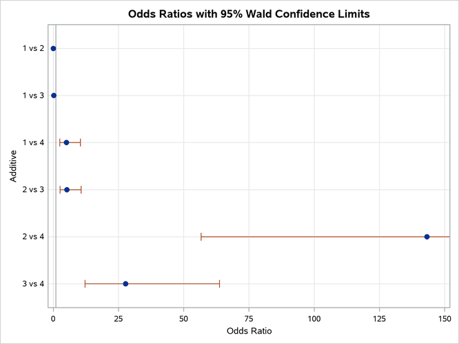
The odds ratio results in Output 79.3.2 show the preferences more clearly. For example, the "Additive 1 vs 4" odds ratio says that the first additive has 5.017 times the odds of receiving a lower score than the fourth additive; that is, the first additive is 5.017 times more likely than the fourth additive to receive a lower score. Output 79.3.3 displays the odds ratios graphically; the range of the confidence limits is truncated by the RANGE=CLIP option, so you can see that "1" is not contained in any of the intervals.
Output 79.3.2: Odds Ratios of All Pairs of Additive Levels
| Odds Ratio Estimates and Wald Confidence Intervals | |||
|---|---|---|---|
| Odds Ratio | Estimate | 95% Confidence Limits | |
| Additive 1 vs 2 | 0.035 | 0.015 | 0.080 |
| Additive 1 vs 3 | 0.181 | 0.087 | 0.376 |
| Additive 1 vs 4 | 5.017 | 2.393 | 10.520 |
| Additive 2 vs 3 | 5.165 | 2.482 | 10.746 |
| Additive 2 vs 4 | 143.241 | 56.558 | 362.777 |
| Additive 3 vs 4 | 27.734 | 12.055 | 63.805 |
Output 79.3.3: Plot of Odds Ratios for Additive
The estimated covariance matrix of the parameters is displayed in Output 79.3.4.
Output 79.3.4: Estimated Covariance Matrix
| Estimated Covariance Matrix | |||||||||||
|---|---|---|---|---|---|---|---|---|---|---|---|
| Parameter | Intercept_1 | Intercept_2 | Intercept_3 | Intercept_4 | Intercept_5 | Intercept_6 | Intercept_7 | Intercept_8 | Additive1 | Additive2 | Additive3 |
| Intercept_1 | 0.316291 | 0.219581 | 0.176278 | 0.147694 | 0.114024 | 0.091085 | 0.057814 | 0.041304 | -0.09419 | -0.18686 | -0.13565 |
| Intercept_2 | 0.219581 | 0.226095 | 0.177806 | 0.147933 | 0.11403 | 0.091081 | 0.057813 | 0.041304 | -0.09421 | -0.18161 | -0.13569 |
| Intercept_3 | 0.176278 | 0.177806 | 0.182473 | 0.148844 | 0.114092 | 0.091074 | 0.057807 | 0.0413 | -0.09427 | -0.1687 | -0.1352 |
| Intercept_4 | 0.147694 | 0.147933 | 0.148844 | 0.152235 | 0.114512 | 0.091109 | 0.05778 | 0.041277 | -0.09428 | -0.14717 | -0.13118 |
| Intercept_5 | 0.114024 | 0.11403 | 0.114092 | 0.114512 | 0.117713 | 0.091821 | 0.057721 | 0.041162 | -0.09246 | -0.11415 | -0.11207 |
| Intercept_6 | 0.091085 | 0.091081 | 0.091074 | 0.091109 | 0.091821 | 0.09522 | 0.058312 | 0.041324 | -0.08521 | -0.09113 | -0.09122 |
| Intercept_7 | 0.057814 | 0.057813 | 0.057807 | 0.05778 | 0.057721 | 0.058312 | 0.07064 | 0.04878 | -0.06041 | -0.05781 | -0.05802 |
| Intercept_8 | 0.041304 | 0.041304 | 0.0413 | 0.041277 | 0.041162 | 0.041324 | 0.04878 | 0.109562 | -0.04436 | -0.0413 | -0.04143 |
| Additive1 | -0.09419 | -0.09421 | -0.09427 | -0.09428 | -0.09246 | -0.08521 | -0.06041 | -0.04436 | 0.142715 | 0.094072 | 0.092128 |
| Additive2 | -0.18686 | -0.18161 | -0.1687 | -0.14717 | -0.11415 | -0.09113 | -0.05781 | -0.0413 | 0.094072 | 0.22479 | 0.132877 |
| Additive3 | -0.13565 | -0.13569 | -0.1352 | -0.13118 | -0.11207 | -0.09122 | -0.05802 | -0.04143 | 0.092128 | 0.132877 | 0.180709 |
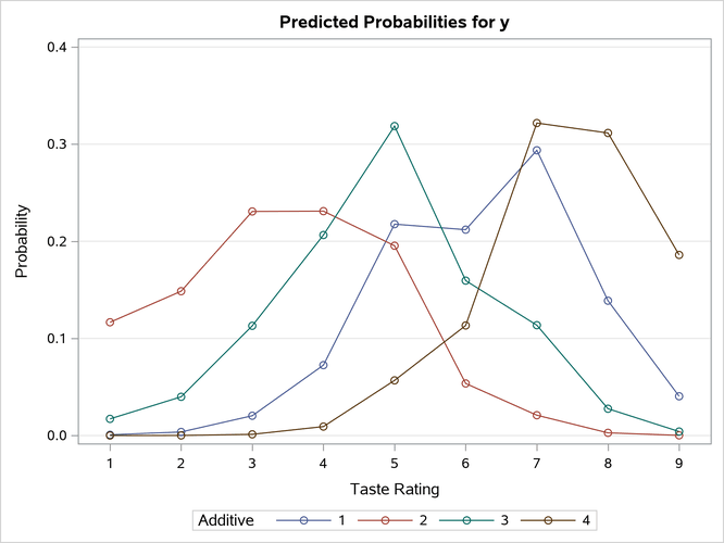
Output 79.3.5 displays the probability of each taste rating y within each additive. You can see that Additive=1 mostly receives ratings of 5 to 7, Additive=2 mostly receives ratings of 2 to 5, Additive=3 mostly receives ratings of 4 to 6, and Additive=4 mostly receives ratings of 7 to 9, which also confirms the previously discussed preference orderings.
Output 79.3.5: Model-Predicted Probabilities
Alternatively, you can use an adjacent-category logit model. The following statements invoke PROC LOGISTIC to fit this model:
proc logistic data=Cheese
   plots(only)=effect(x=y sliceby=additive connect yrange=(0,0.4));
   freq freq;
   class Additive (param=ref ref='4');
   model y=Additive / nooddsratio link=alogit;
   oddsratio Additive;
   title 'Multiple Response Cheese Tasting Experiment';
run;
You can see that the parameter estimates for the intercepts in Output 79.3.6 are no longer strictly increasing, as they are for the cumulative model in Output 79.3.1.
Output 79.3.6: Adjacent-Category Logistic Regression Analysis
| Multiple Response Cheese Tasting Experiment |
| Analysis of Maximum Likelihood Estimates | ||||||
|---|---|---|---|---|---|---|
| Parameter | DF | Estimate | Standard Error |
Wald Chi-Square |
Pr > ChiSq | |
| Intercept | 1 | 1 | -2.2262 | 0.5542 | 16.1350 | <.0001 |
| Intercept | 2 | 1 | -2.4238 | 0.4620 | 27.5216 | <.0001 |
| Intercept | 3 | 1 | -1.9852 | 0.3800 | 27.2909 | <.0001 |
| Intercept | 4 | 1 | -1.8164 | 0.3294 | 30.4096 | <.0001 |
| Intercept | 5 | 1 | -0.6908 | 0.3097 | 4.9737 | 0.0257 |
| Intercept | 6 | 1 | -1.0433 | 0.2841 | 13.4902 | 0.0002 |
| Intercept | 7 | 1 | 0.0322 | 0.2667 | 0.0146 | 0.9040 |
| Intercept | 8 | 1 | 0.5160 | 0.3527 | 2.1402 | 0.1435 |
| Additive | 1 | 1 | 0.7172 | 0.1783 | 16.1776 | <.0001 |
| Additive | 2 | 1 | 1.9838 | 0.2463 | 64.8748 | <.0001 |
| Additive | 3 | 1 | 1.3826 | 0.2122 | 42.4478 | <.0001 |
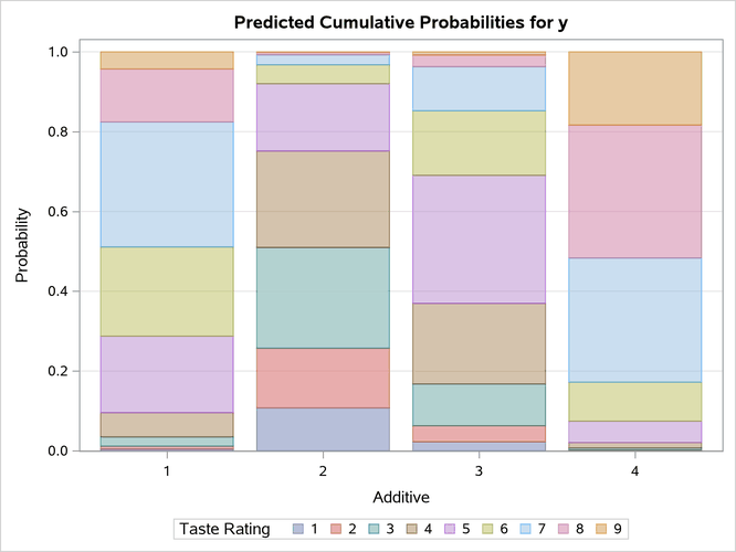
The odds ratio results in Output 79.3.7 show the same preferences that you obtain from the proportional odds model. Output 79.3.8 displays the probability of each additive according to the taste rating.
Output 79.3.7: Odds Ratios of All Pairs of Additive Levels
| Odds Ratio Estimates and Wald Confidence Intervals | |||
|---|---|---|---|
| Odds Ratio | Estimate | 95% Confidence Limits | |
| Additive 1 vs 2 | 0.282 | 0.192 | 0.414 |
| Additive 1 vs 3 | 0.514 | 0.377 | 0.700 |
| Additive 1 vs 4 | 2.049 | 1.444 | 2.906 |
| Additive 2 vs 3 | 1.824 | 1.355 | 2.456 |
| Additive 2 vs 4 | 7.271 | 4.487 | 11.782 |
| Additive 3 vs 4 | 3.985 | 2.629 | 6.040 |
Output 79.3.8: Model-Predicted Probabilities