The LOGISTIC Procedure
Example 79.7 ROC Curve, Customized Odds Ratios, Goodness-of-Fit Statistics, R-Square, and Confidence Limits
(View the complete code for this example.)
This example plots an ROC curve, estimates a customized odds ratio, produces the traditional goodness-of-fit analysis, displays the generalized R-square measures for the fitted model, calculates the normal confidence intervals for the regression parameters, and produces a display of the probability function and prediction curves for the fitted model. The data consist of three variables: n (number of subjects in the sample), disease (number of diseased subjects in the sample), and age (age for the sample). A linear logistic regression model is used to study the effect of age on the probability of contracting the disease. The statements to produce the data set and perform the analysis are as follows:
data Data1;
   input disease n age id $;
   datalines;
 0 14 25 a
 0 20 35 b
 0 19 45 c
 7 18 55 d
 6 12 65 e
17 17 75 f
;
ods graphics on;
%let _ROC_XAXISOPTS_LABEL=False Positive Fraction;
%let _ROC_YAXISOPTS_LABEL=True Positive Fraction;
proc logistic data=Data1 plots(only)=roc(id=id);
   model disease/n=age / scale=none
                         clparm=wald
                         clodds=pl
                         rsquare;
   units age=10;
   id id;
   effectplot;
run;
%symdel _ROC_XAXISOPTS_LABEL _ROC_YAXISOPTS_LABEL;
The option SCALE=NONE is specified to produce the deviance and Pearson goodness-of-fit analysis without adjusting for overdispersion. The RSQUARE option is specified to produce generalized R-square measures of the fitted model. The CLPARM=WALD option is specified to produce the Wald confidence intervals for the regression parameters. The UNITS statement is specified to produce customized odds ratio estimates for a change of 10 years in the age variable, and the CLODDS=PL option is specified to produce profile-likelihood confidence limits for the odds ratio. The PLOTS= option with ODS Graphics enabled produces a graphical display of the ROC curve with certain points labeled with their ID values, the two macro variables modify the ROC axis labels, and the EFFECTPLOT statement displays the model fit.
The results in Output 79.7.1 show that the deviance and Pearson statistics indicate no lack of fit in the model.
Output 79.7.1: Deviance and Pearson Goodness-of-Fit Analysis
| Deviance and Pearson Goodness-of-Fit Statistics | ||||
|---|---|---|---|---|
| Criterion | Value | DF | Value/DF | Pr > ChiSq |
| Deviance | 7.7756 | 4 | 1.9439 | 0.1002 |
| Pearson | 6.6020 | 4 | 1.6505 | 0.1585 |
| Number of events/trials observations: 6 |
Output 79.7.2 shows that the R-square for the model is 0.74. The odds of an event increases by a factor of 7.9 for each 10-year increase in age.
Output 79.7.2: R-Square, Confidence Intervals, and Customized Odds Ratio
| Model Fit Statistics | |||
|---|---|---|---|
| Criterion | Intercept Only | Intercept and Covariates | |
| Log Likelihood | Full Log Likelihood | ||
| AIC | 124.173 | 52.468 | 18.075 |
| SC | 126.778 | 57.678 | 23.285 |
| -2 Log L | 122.173 | 48.468 | 14.075 |
| R-Square | 0.5215 | Max-rescaled R-Square | 0.8925 |
|---|
| Testing Global Null Hypothesis: BETA=0 | |||
|---|---|---|---|
| Test | Chi-Square | DF | Pr > ChiSq |
| Likelihood Ratio | 73.7048 | 1 | <.0001 |
| Score | 55.3274 | 1 | <.0001 |
| Wald | 23.3475 | 1 | <.0001 |
| Analysis of Maximum Likelihood Estimates | |||||
|---|---|---|---|---|---|
| Parameter | DF | Estimate | Standard Error |
Wald Chi-Square |
Pr > ChiSq |
| Intercept | 1 | -12.5016 | 2.5555 | 23.9317 | <.0001 |
| age | 1 | 0.2066 | 0.0428 | 23.3475 | <.0001 |
| Association of Predicted Probabilities and Observed Responses |
|||
|---|---|---|---|
| Percent Concordant | 92.6 | Somers' D | 0.906 |
| Percent Discordant | 2.0 | Gamma | 0.958 |
| Percent Tied | 5.4 | Tau-a | 0.384 |
| Pairs | 2100 | c | 0.953 |
| Parameter Estimates and Wald Confidence Intervals |
|||
|---|---|---|---|
| Parameter | Estimate | 95% Confidence Limits | |
| Intercept | -12.5016 | -17.5104 | -7.4929 |
| age | 0.2066 | 0.1228 | 0.2904 |
| Odds Ratio Estimates and Profile-Likelihood Confidence Intervals |
||||
|---|---|---|---|---|
| Effect | Unit | Estimate | 95% Confidence Limits | |
| age | 10.0000 | 7.892 | 3.881 | 21.406 |
Because ODS Graphics is enabled, a graphical display of the ROC curve is produced as shown in Output 79.7.3.
Output 79.7.3: Receiver Operating Characteristic Curve
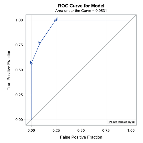
Note that the area under the ROC curve is estimated by the statistic c in the "Association of Predicted Probabilities and Observed Responses" table. In this example, the area under the ROC curve is 0.953. By default, the Y axis is labeled "Sensitivity" and the X axis is labeled "1–Specificity".
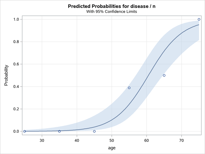
Because there is only one continuous covariate and because ODS Graphics is enabled, the EFFECTPLOT statement produces a graphical display of the predicted probability curve with bounding 95% confidence limits as shown in Output 79.7.4.
Output 79.7.4: Predicted Probability and 95% Prediction Limits