Statistical Graphics Using ODS
The EFFECT and EFFECTPLOT Statements
Splines are available in many other procedures when you use the EFFECT statement. The following procedures provide an EFFECT statement: GEE, GENMOD, GLIMMIX, GLMSELECT, HPMIXED, LOGISTIC, ORTHOREG, PHREG, PLM, PROBIT, QUANTLIFE, QUANTREG, QUANTSELECT, ROBUSTREG, SURVEYLOGISTIC, and SURVEYREG.
B-Spline Fit Function
The following step fits a spline that has five equally spaced knots:
proc orthoreg data=sashelp.heart;
   effect spl = spline(height / knotmethod=equal(5));
   model weight = spl;
   effectplot / obs;
run;
The EFFECT statement names the variable Height as a SPLINE variable and requests five evenly spaced knots. The name in the EFFECT statement, Spl, is then specified in the MODEL statement. Notice that the method is similar to the method in PROC TRANSREG, even though elements of the syntax are different. The EFFECTPLOT statement displays the fit function, and the OBS option adds the scatter plot to the graph. Note that the plot-type, which can appear before the slash, is not specified. The results are displayed in Output 24.6.22.
Output 24.6.22: EFFECT and EFFECTPLOT Statements
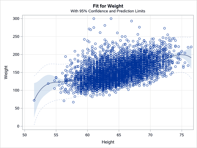
B-Spline Fit Functions
The EFFECTPLOT statement acts like PROC SGPLOT in that it automatically adds observations for interpolation (and in some cases extrapolation). The following step creates the plot in Output 24.6.23:
proc orthoreg data=sashelp.gas;
   effect spl = spline(eqratio / knotmethod=equal(3));
   class fuel;
   model nox = spl | fuel;
   effectplot / obs extend=data;
   ods output SliceFitPlot=sp;
run;
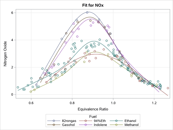
Output 24.6.23: EFFECT and EFFECTPLOT Statements with a CLASS Variable

Note that the plot-type, which can appear before the slash, must not be specified for an interaction model like this. Furthermore, you must specify the EXTEND=DATA option for this type of plot. It causes the interpolation for plotted values to be between the minimum and maximum for each CLASS level, as is shown in the example that created the plot in Output 24.6.15. Without this option, the function for each group is generated through the range of the minimum and maximum of the spline variable EqRatio. Splines often rapidly head to plus or minus infinity as you extrapolate beyond the range of your data. The option does not affect the analysis; it affects only the plot construction. The number of knots was changed to three in this example. Five knots illustrate an even more extreme version of the same problem that was shown in Output 24.6.12. Because the 82rongas function is sparse, that function is not well behaved when there are five knots.
Natural Cubic Splines (Restricted Splines)
You can get much better results by using natural cubic splines (Hastie, Tibshirani, and Friedman 2009), which are also known as restricted splines. The following step creates the plot in Output 24.6.24:
proc orthoreg data=sashelp.gas;
   effect spl = spline(eqratio / naturalcubic knotmethod=equal(5));
   class fuel;
   model nox = spl | fuel;
   effectplot / obs;
run;
Output 24.6.24: Natural Cubic (Restricted) Splines
Restricted splines are linear beyond the interior knots, so they tend to be better behaved at the tails, particularly with a sparse CLASS level such as 82rongas. There are 30 parameters in this restricted-spline model. In contrast, the full spline model has 51 parameters.