The PSMATCH Procedure
Example 101.1 Propensity Score Weighting
(View the complete code for this example.)
This example illustrates how you can create observation weights that are appropriate for estimating the average treatment effect (ATE) in a subsequent outcome analysis (the outcome analysis itself is not shown here).
The data for this example are observations on patients in a nonrandomized clinical trial. The trial and the Drugs data set that contains the patient information are described in the section Getting Started: PSMATCH Procedure.
The following statements specify a logistic regression model for obtaining propensity scores, compute observation weights from the propensity scores, request statistics and plots for balance assessment, and save the weights in an output data set:
ods graphics on;
proc psmatch data=drugs region=allobs;
   class Drug Gender;
   psmodel Drug(Treated='Drug_X')= Gender Age BMI;
   psweight weight=atewgt nlargestwgt=6;
   assess lps var=(Gender Age BMI)
          / varinfo plots=(barchart boxplot(display=(lps BMI)) wgtcloud);
   id BMI;
   output out(obs=all)=OutEx1 weight=_ATEWgt_;
run;
The PSMODEL statement specifies the logistic regression model that creates the propensity score for each observation, which is the probability that the patient receives Drug_X. The CLASS statement specifies the classification variables in the model. The Drug variable is the binary treatment indicator variable, and TREATED='Drug_X' identifies Drug_X as the treated group. The Gender, Age, and BMI variables are included in the model because they are believed to be related to the assignment. The REGION=ALLOBS option specifies that the support region contains all observations. Weights are computed for all observations, regardless of the REGION= option.
The "Data Information" table in Output 101.1.1 displays the numbers of observations in the treated and control groups, the lower and upper limits of the propensity scores for observations in the support region, and the numbers of observations in the treated and control groups that fall within the support region. Because REGION=ALLOBS is specified, the lower and upper limits for of the propensity scores for observations in the support region are the minimum and maximum of the propensity scores for all observations. Consequently, all 373 observations in the control group fall within the support region, and all 133 observations in the treated group fall within the support region.
Output 101.1.1: Data Information
| Data Information | |
|---|---|
| Data Set | WORK.DRUGS |
| Output Data Set | WORK.OUTEX1 |
| Treatment Variable | Drug |
| Treated Group | Drug_X |
| All Obs (Treated) | 113 |
| All Obs (Control) | 373 |
| Support Region | All Obs |
| Lower PS Support | 0.020157 |
| Upper PS Support | 0.685757 |
| Support Region Obs (Treated) | 113 |
| Support Region Obs (Control) | 373 |
The "Propensity Score Information" table in Output 101.1.2 displays summary statistics by treatment group for all observations (labeled "All"), for observations in the support region (labeled "Region"), and for weighted observations in the support region (labeled "Weighted"). Because the support region consists of all observations, the first two rows in the table are identical. The WEIGHT=ATEWGT option in the PSWEIGHT statement displays summary statistics for ATE weighted observations.
Output 101.1.2: Propensity Score Information
| Propensity Score Information | |||||||||||||
|---|---|---|---|---|---|---|---|---|---|---|---|---|---|
| Observations | Treated (Drug = Drug_X) | Control (Drug = Drug_A) | Treated - Control |
||||||||||
| N | Weight | Mean | Standard Deviation |
Minimum | Maximum | N | Weight | Mean | Standard Deviation |
Minimum | Maximum | Mean Difference |
|
| All | 113 | 0.3108 | 0.1325 | 0.0602 | 0.6411 | 373 | 0.2088 | 0.1320 | 0.0202 | 0.6858 | 0.1020 | ||
| Region | 113 | 0.3108 | 0.1325 | 0.0602 | 0.6411 | 373 | 0.2088 | 0.1320 | 0.0202 | 0.6858 | 0.1020 | ||
| Weighted | 113 | 460.45 | 0.2454 | 0.1268 | 0.0602 | 0.6411 | 373 | 489.59 | 0.2381 | 0.1496 | 0.0202 | 0.6858 | 0.0073 |
The ASSESS statement produces tables and plots, shown in Output 101.1.3 through Output 101.1.5 and in Output 101.1.7 through Output 101.1.10, that summarize differences in the distributions of specified variables between treated and control groups. As requested by the LPS and VAR= options, these variables are the logit of the propensity score and the data variables Gender, Age, and BMI. Differences are summarized for all observations and for observations in the support region. Again, these two sets of differences are identical because REGION=ALLOBS is specified. The WEIGHT=ATEWGT option in the PSWEIGHT statement requests that differences in the variables also be summarized for the weighted observations. By comparing the differences for weighted observations to the differences for observations in the support region, you can assess how well weighting improves the balance for each variable.
The VARINFO option requests the "Variable Information" table, shown in Output 101.1.3, which displays variable summary statistics and differences between the treated and control groups for all observations (labeled "All"), for observations in the support region (labeled "Region"), and for weighted observations (labeled "Weighted"). For the binary classification variable (Gender), the difference is in the proportion of the first ordered level (Female).
Output 101.1.3: Variable Information
| Variable Information | ||||||||||||||
|---|---|---|---|---|---|---|---|---|---|---|---|---|---|---|
| Variable | Observations | Treated (Drug = Drug_X) | Control (Drug = Drug_A) | Treated - Control |
||||||||||
| N | Weight | Mean | Standard Deviation |
Minimum | Maximum | N | Weight | Mean | Standard Deviation |
Minimum | Maximum | Mean Difference |
||
| Logit Prop Score | All | 113 | -0.88062 | 0.681761 | -2.74745 | 0.58035 | 373 | -1.52059 | 0.844486 | -3.88386 | 0.78036 | 0.63997 | ||
| Region | 113 | -0.88062 | 0.681761 | -2.74745 | 0.58035 | 373 | -1.52059 | 0.844486 | -3.88386 | 0.78036 | 0.63997 | |||
| Weighted | 113 | 460.45 | -1.25406 | 0.741386 | -2.74745 | 0.58035 | 373 | 489.59 | -1.35103 | 0.894234 | -3.88386 | 0.78036 | 0.09698 | |
| Age | All | 113 | 36.30973 | 5.534114 | 26.00000 | 49.00000 | 373 | 40.40483 | 6.579103 | 25.00000 | 57.00000 | -4.09509 | ||
| Region | 113 | 36.30973 | 5.534114 | 26.00000 | 49.00000 | 373 | 40.40483 | 6.579103 | 25.00000 | 57.00000 | -4.09509 | |||
| Weighted | 113 | 460.45 | 38.59813 | 5.773228 | 26.00000 | 49.00000 | 373 | 489.59 | 39.32670 | 6.771606 | 25.00000 | 57.00000 | -0.72857 | |
| BMI | All | 113 | 24.49257 | 1.863797 | 20.33000 | 28.34000 | 373 | 23.75327 | 1.980778 | 19.22000 | 28.61000 | 0.73930 | ||
| Region | 113 | 24.49257 | 1.863797 | 20.33000 | 28.34000 | 373 | 23.75327 | 1.980778 | 19.22000 | 28.61000 | 0.73930 | |||
| Weighted | 113 | 460.45 | 24.03522 | 1.896607 | 20.33000 | 28.34000 | 373 | 489.59 | 23.95492 | 2.004019 | 19.22000 | 28.61000 | 0.08030 | |
| Gender | All | 113 | 0.43363 | 0.495575 | 373 | 0.45845 | 0.498270 | -0.02482 | ||||||
| Region | 113 | 0.43363 | 0.495575 | 373 | 0.45845 | 0.498270 | -0.02482 | |||||||
| Weighted | 113 | 460.45 | 0.47335 | 0.499289 | 373 | 489.59 | 0.45479 | 0.497952 | 0.01856 | |||||
The statistics in Output 101.1.3 are identical for all observations and for observations in the support region because REGION=ALLOBS is specified.
As indicated in the column labeled Weight, the total weight of the treated units is 460.45 and the total weight of the control units is 489.59, which are close to 486, the total number of units. The weights are ATE weights because WEIGHT=ATEWGT is specified in the PSWEIGHT statement. For information about ATE weights, see the section Inverse Probability of Treatment Weighting.
Note that in comparison to the unweighted means, the weighted means for the control units are closer in absolute value to the corresponding weighted means for the treated units.
The "Standardized Mean Differences" table, shown in Output 101.1.4, displays standardized mean differences in the variables between the treated and control groups, based on all observations, on observations in the support region, and on weighted observations.
Output 101.1.4: Standardized Mean Differences
| Standardized Mean Differences (Treated - Control) | ||||||
|---|---|---|---|---|---|---|
| Variable | Observations | Mean Difference |
Standard Deviation |
Standardized Difference |
Percent Reduction |
Variance Ratio |
| Logit Prop Score | All | 0.63997 | 0.767449 | 0.83389 | 0.6517 | |
| Region | 0.63997 | 0.83389 | 0.00 | 0.6517 | ||
| Weighted | 0.09698 | 0.12636 | 84.85 | 0.6874 | ||
| Age | All | -4.09509 | 6.079104 | -0.67363 | 0.7076 | |
| Region | -4.09509 | -0.67363 | 0.00 | 0.7076 | ||
| Weighted | -0.72857 | -0.11985 | 82.21 | 0.7269 | ||
| BMI | All | 0.73930 | 1.923178 | 0.38441 | 0.8854 | |
| Region | 0.73930 | 0.38441 | 0.00 | 0.8854 | ||
| Weighted | 0.08030 | 0.04175 | 89.14 | 0.8957 | ||
| Gender | All | -0.02482 | 0.496925 | -0.04994 | 0.9892 | |
| Region | -0.02482 | -0.04994 | 0.00 | 0.9892 | ||
| Weighted | 0.01856 | 0.03735 | 25.21 | 1.0054 | ||
| Standard deviation of All observations used to compute standardized differences | ||||||
The standardized mean differences based on weighted observations are significantly reduced; the largest of these differences is 0.12637 in absolute value, which is less than the upper limit of 0.25 that is recommended by Rubin (2001, p. 174) and Stuart (2010, p. 11). The treated-to-control variance ratios between the two groups are within the recommended range of 0.5 to 2. The percentage of reduction in variable mean difference is 0 for observations in the support region because REGION=ALLOBS is specified.
The PSMATCH procedure displays a standardized mean differences plot, shown in Output 101.1.5, for the variables that are specified in the ASSESS statement.
Output 101.1.5: Standardized Mean Differences Plot
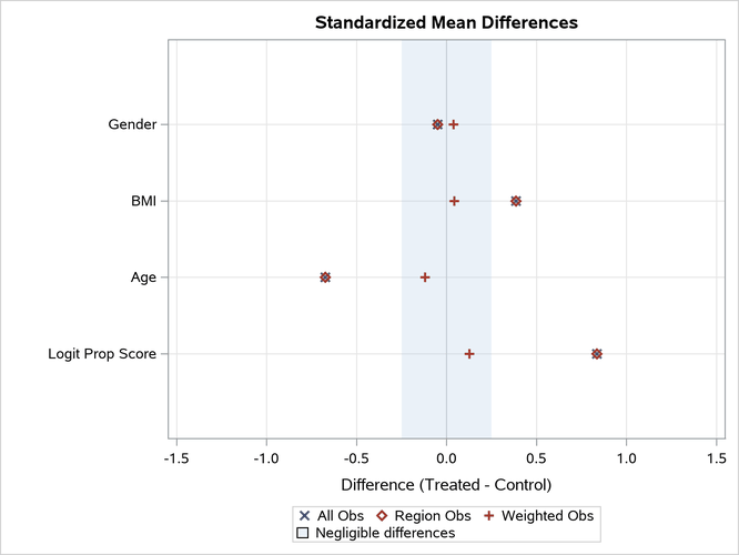
The "Standardized Mean Differences Plot" displays the differences that are shown in the "Standardized Mean Differences" table in Output 101.1.4. All differences for the weighted observations are within the recommended limits of –0.25 and 0.25, which are indicated by the shaded area.
The NLARGESTWGT=6 option displays the "Observations with Largest Weights" table, shown in Output 101.1.6, which lists the observations that have the six largest weights in the treated and control groups.
Output 101.1.6: Observations with Largest Weights
| Observations with Largest IPTW-ATE Weights | |||||||
|---|---|---|---|---|---|---|---|
| Treated (Drug = Drug_X) | Control (Drug = Drug_A) | ||||||
| Expected Weight = 4.3009 | Expected Weight = 1.3029 | ||||||
| Observation | BMI | Weight | Scaled Weight |
Observation | BMI | Weight | Scaled Weight |
| 202 | 20.75 | 16.60 | 3.86 | 317 | 28.61 | 3.18 | 2.44 |
| 479 | 22.22 | 14.79 | 3.44 | 134 | 28.07 | 3.15 | 2.42 |
| 250 | 23.96 | 11.40 | 2.65 | 437 | 25.76 | 2.74 | 2.10 |
| 227 | 21.11 | 11.23 | 2.61 | 417 | 26.81 | 2.62 | 2.01 |
| 274 | 24.17 | 9.69 | 2.25 | 446 | 27.75 | 2.62 | 2.01 |
| 174 | 23.56 | 9.02 | 2.10 | 81 | 27.20 | 2.40 | 1.84 |
In the table, the scaled weights (which are the weights divided by their expected weights) are also displayed for ease of comparison. For more information about the expected weights in the treated and control group, see the section Propensity Score Weighting.
The PLOTS=WGTCLOUD option displays a cloud plot for the stabilized weights, which is shown in Output 101.1.7. This plot is called a cloud plot because the points are jittered in the vertical direction in order to avoid overplotting.
Output 101.1.7: Weight Cloud Plot
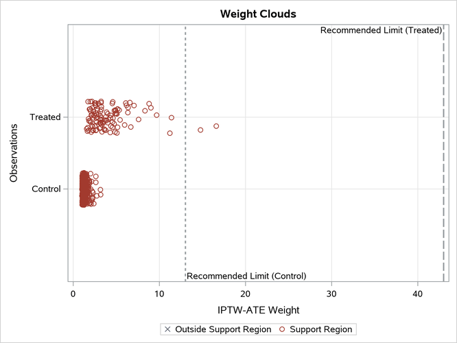
By default, the plot displays reference lines that represent 10 times the expected ATE weights in the treated and control groups. For information about these average weights, see the section Inverse Probability of Treatment Weighting.
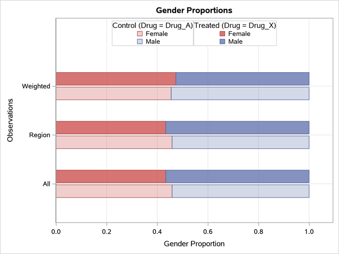
The PLOTS=BARCHART option displays a bar chart for each classification variable that is specified in the ASSESS statement. As shown in Output 101.1.8, the bar chart shows the distributions of Gender based on all observations, on observations in the support region, and on weighted observations. By default, the bar chart displays the proportions of levels of Gender. Weighting the observations makes a slight improvement in the balance between males and females.
Output 101.1.8: Gender Bar Chart
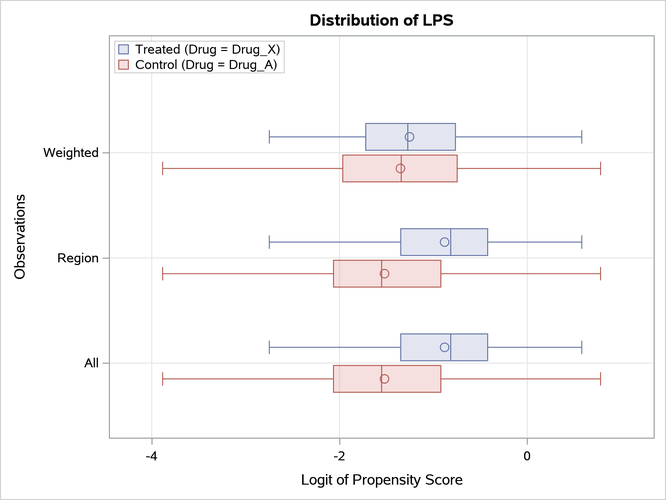
The PLOTS=BOXPLOT(DISPLAY=(LPS BMI)) option displays box plots for LPS and BMI, as shown in Output 101.1.9 and Output 101.1.10, respectively. These plots compare the distributions of the variables for the treated and control groups. Weighting the observations makes a good improvement in the balance between males and females.
Output 101.1.9: LPS Box Plot
Output 101.1.10: BMI Box Plot
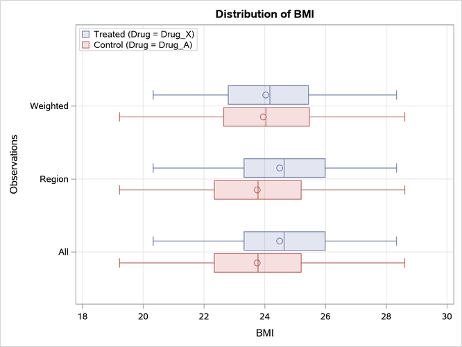
Because there is good balance in the weighted distributions of the variables Gender, Age, and BMI, the observations and their weights can be saved in an output data set for use in a subsequent outcome analysis.
In situations where you are not satisfied with the variable balance, you can do one or more of the following to improve the balance: you can select another set of variables to fit the propensity score model, you can modify the specification of the propensity score model by using nonlinear terms for the continuous variables or by adding interactions (Rosenbaum and Rubin 1984), or you can choose another propensity score method (such as matching).
The OUT(OBS=ALL)=OutEx1 option in the OUTPUT statement creates an output data set, OutEx1, that contains all available observations. The following statements list the first 10 observations in OutEx1, as shown in Output 101.1.11.
proc print data=OutEx1(obs=10);
   var PatientID Drug Gender Age BMI _ps_ _AteWgt_;
run;
Output 101.1.11: Output Data Set with ATE Weights
| Obs | PatientID | Drug | Gender | Age | BMI | _PS_ | _ATEWgt_ |
|---|---|---|---|---|---|---|---|
| 1 | 284 | Drug_X | Male | 29 | 22.02 | 0.36444 | 2.74397 |
| 2 | 201 | Drug_A | Male | 45 | 26.68 | 0.22296 | 1.28694 |
| 3 | 147 | Drug_A | Male | 42 | 21.84 | 0.11323 | 1.12768 |
| 4 | 307 | Drug_X | Male | 38 | 22.71 | 0.19733 | 5.06767 |
| 5 | 433 | Drug_A | Male | 31 | 22.76 | 0.35311 | 1.54586 |
| 6 | 435 | Drug_A | Male | 43 | 26.86 | 0.27263 | 1.37482 |
| 7 | 159 | Drug_A | Female | 45 | 25.47 | 0.14911 | 1.17523 |
| 8 | 368 | Drug_A | Female | 49 | 24.28 | 0.07780 | 1.08437 |
| 9 | 286 | Drug_A | Male | 31 | 23.31 | 0.38341 | 1.62182 |
| 10 | 163 | Drug_X | Female | 39 | 25.34 | 0.24995 | 4.00073 |
By default, the output data set includes the variable _PS_, which provides the propensity score. The weight for each treated unit is computed as 1 / p and the weight for each control unit is computed as 1 / (1 – p), where p is the propensity score.
After the responses for the trial are observed, they can be added to the data set OutEx1 as the starting point for an outcome analysis. Assuming that no other confounding variables are associated with both the response variable and the treatment group indicator Drug, you can estimate the ATE by performing a weighted version of the outcome analysis that you would have used to estimate the treatment effect if the original data set had resulted from a randomized trial.