The PSMATCH Procedure
Example 101.2 Propensity Score Stratification
(View the complete code for this example.)
This example illustrates how you can stratify observations based on their propensity scores, so that the stratified observations can be used to estimate the treatment effect in a subsequent outcome analysis (the outcome analysis is not shown here).
The data for this example are observations on patients in a nonrandomized clinical trial. The trial and the Drugs data set that contains the patient information are described in the section Getting Started: PSMATCH Procedure.
The following statements create five strata that are based on propensity scores:
ods graphics on;
proc psmatch data=drugs region=allobs;
   class Drug Gender;
   psmodel Drug(Treated='Drug_X')= Gender Age BMI;
   strata nstrata=5 key=treated stratumwgt=total;
   assess ps var=(Gender BMI)
          / varinfo plots=(barchart cdfplot);
   output out(obs=all)=OutEx2;
run;
The PSMODEL statement specifies the logistic regression model that creates the propensity score for each observation, which is the probability that the patient receives Drug_X. The CLASS statement specifies the classification variables in the model. The Drug variable is the binary treatment indicator variable, and TREATED='Drug_X' identifies Drug_X as the treated group. The Gender, Age, and BMI variables are included in the model because they are believed to be related to the assignment.
The PSMATCH procedure stratifies the observations whose propensity scores lie in the support region that is specified in the REGION= option. The REGION=ALLOBS option requests that all observations be stratified.
The STRATA statement creates strata of observations based on their propensity scores. The NSTRATA=5 option (which is the default) stratifies the observations into five strata and the KEY=TREATED option (which is the default) requests that each stratum contain approximately the same number of treated observations.
The "Data Information" table in Output 101.2.1 displays the numbers of observations in the treated and control groups, the lower and upper limits of the propensity scores for observations in the support region, and the numbers of observations in the treated and control groups that fall within the support region. Because REGION=ALLOBS is specified, the lower and upper limits of the propensity scores for observations in the support region are simply the minimum and maximum of the propensity scores for all observations. Likewise, all 373 observations in the control group fall within the support region.
Output 101.2.1: Data Information
| Data Information | |
|---|---|
| Data Set | WORK.DRUGS |
| Output Data Set | WORK.OUTEX2 |
| Treatment Variable | Drug |
| Treated Group | Drug_X |
| All Obs (Treated) | 113 |
| All Obs (Control) | 373 |
| Support Region | All Obs |
| Lower PS Support | 0.020157 |
| Upper PS Support | 0.685757 |
| Support Region Obs (Treated) | 113 |
| Support Region Obs (Control) | 373 |
| Number of Strata | 5 |
The "Propensity Score Information" table in Output 101.2.2 displays summary statistics for the treated and control groups. Statistics are computed for all observations, for observations in the support region, and for strata. The first two rows of statistics are identical because REGION=ALLOBS is specified.
Output 101.2.2: Propensity Score Information
| Propensity Score Information | |||||||||||
|---|---|---|---|---|---|---|---|---|---|---|---|
| Observations | Treated (Drug = Drug_X) | Control (Drug = Drug_A) | Treated - Control |
||||||||
| N | Mean | Standard Deviation |
Minimum | Maximum | N | Mean | Standard Deviation |
Minimum | Maximum | Mean Difference |
|
| All | 113 | 0.3108 | 0.1325 | 0.0602 | 0.6411 | 373 | 0.2088 | 0.1320 | 0.0202 | 0.6858 | 0.1020 |
| Region | 113 | 0.3108 | 0.1325 | 0.0602 | 0.6411 | 373 | 0.2088 | 0.1320 | 0.0202 | 0.6858 | 0.1020 |
| Strata | 5 | 0.2426 | 0.0212 | 0.1404 | 0.5121 | 5 | 0.2318 | 0.0227 | 0.1159 | 0.5312 | 0.0107 |
Note that for strata, the displayed statistics refer to the strata rather than to the observational units. These statistics are the number of strata, the weighted mean of the stratum means, the standard deviation of this weighted mean, and the minimum and maximum of these stratum means. The weights for computing the weighted mean are the stratum weights (as shown in the last column of Output 101.2.3), which are proportions of total units (treated and control units combined) in strata by the default STRATUMWGT=TOTAL option.
When you specify a STRATA statement, the "Strata Information" table, which is shown in Output 101.2.3, displays the following information for each stratum: the minimum and maximum propensity scores, the number of observations in the treatment group, the number of observations in the control group, the total number of observations, and the stratum weight.
Output 101.2.3: Strata Information
| Strata Information | ||||||
|---|---|---|---|---|---|---|
| Stratum Index |
Frequencies | Stratum Weight |
||||
| Propensity Score Range | Treated | Control | Total | |||
| 1 | 0.0202 | 0.1944 | 22 | 209 | 231 | 0.475 |
| 2 | 0.1967 | 0.2613 | 23 | 59 | 82 | 0.169 |
| 3 | 0.2619 | 0.3223 | 23 | 38 | 61 | 0.126 |
| 4 | 0.3259 | 0.4342 | 23 | 41 | 64 | 0.132 |
| 5 | 0.4379 | 0.6858 | 22 | 26 | 48 | 0.099 |
The table shows that each stratum contains approximately the same number of observations for treated units, as requested by the KEY=TREATED option. In addition, there are enough control units in each stratum to ensure a reliable estimate of the treatment effect for this stratum, even though the propensity score distributions in the treated and control groups are different.
The ASSESS statement produces tables and plots, shown in Output 101.2.4 through Output 101.2.14, that summarize differences in the distributions of specified variables between treated and control groups. As requested by the PS and VAR= options, these variables are the propensity score and the data variables Gender and BMI. By default, differences are summarized for all observations and for observations in the support region. Again, these two sets of differences are identical because REGION=ALLOBS is specified. When you specify a STRATA statement, differences after stratification are also displayed.
The VARINFO option requests the "Variable Information" table, shown in Output 101.2.4, which displays variable summary statistics and mean differences between the treated and control groups for all observations (labeled "All"), for observations in the support region (labeled "Region"), and for the stratified observations (labeled "Strata"). The first two sets of statistics and mean differences are identical because REGION=ALLOBS is specified. For the binary classification variable (Gender), the difference is in the proportion of the first ordered level (Female).
Output 101.2.4: Variable Information
| Variable Information | ||||||||||||
|---|---|---|---|---|---|---|---|---|---|---|---|---|
| Variable | Observations | Treated (Drug = Drug_X) | Control (Drug = Drug_A) | Treated - Control |
||||||||
| N | Mean | Standard Deviation |
Minimum | Maximum | N | Mean | Standard Deviation |
Minimum | Maximum | Mean Difference |
||
| Prop Score | All | 113 | 0.31077 | 0.132467 | 0.06023 | 0.64115 | 373 | 0.20880 | 0.131969 | 0.02016 | 0.68576 | 0.10197 |
| Region | 113 | 0.31077 | 0.132467 | 0.06023 | 0.64115 | 373 | 0.20880 | 0.131969 | 0.02016 | 0.68576 | 0.10197 | |
| Strata | 5 | 0.24256 | 0.021157 | 0.14040 | 0.51209 | 5 | 0.23182 | 0.022710 | 0.11589 | 0.53118 | 0.01074 | |
| BMI | All | 113 | 24.49257 | 1.863797 | 20.33000 | 28.34000 | 373 | 23.75327 | 1.980778 | 19.22000 | 28.61000 | 0.73930 |
| Region | 113 | 24.49257 | 1.863797 | 20.33000 | 28.34000 | 373 | 23.75327 | 1.980778 | 19.22000 | 28.61000 | 0.73930 | |
| Strata | 5 | 24.08101 | 0.954962 | 23.50091 | 25.69500 | 5 | 23.89531 | 1.019772 | 23.17541 | 25.73077 | 0.18570 | |
| Gender | All | 113 | 0.43363 | 0.495575 | 373 | 0.45845 | 0.498270 | -0.02482 | ||||
| Region | 113 | 0.43363 | 0.495575 | 373 | 0.45845 | 0.498270 | -0.02482 | |||||
| Strata | 5 | 0.44921 | 0.270442 | 5 | 0.45232 | 0.270450 | -0.00311 | |||||
For each variable, the row labeled "Strata" displays the number of strata, the weighted mean of the stratum means, and the standard deviation of this weighted mean, where the weights are computed as proportions of total units (treated and control units combined) in strata by the default STRATUMWGT=TOTAL option. The row also displays the minimum and maximum of the variable averages within the strata.
For each variable, the "Standardized Mean Differences" table in Output 101.2.5 displays the standardized mean differences between the treated and control groups for all observations, for observations in the support region, and for the stratified observations. The sections Weighting after Stratification and Pooled Standardized Mean Differences across the Strata explain how the statistics are computed for the stratified observations.
Output 101.2.5: Standardized Mean Differences
| Standardized Mean Differences (Treated - Control) | ||||||
|---|---|---|---|---|---|---|
| Variable | Observations | Mean Difference |
Standard Deviation |
Standardized Difference |
Percent Reduction |
Variance Ratio |
| Prop Score | All | 0.10197 | 0.132218 | 0.77124 | 1.0076 | |
| Region | 0.10197 | 0.77124 | 0.00 | 1.0076 | ||
| Strata | 0.01074 | 0.08121 | 89.47 | 0.8678 | ||
| BMI | All | 0.73930 | 1.923178 | 0.38441 | 0.8854 | |
| Region | 0.73930 | 0.38441 | 0.00 | 0.8854 | ||
| Strata | 0.18570 | 0.09656 | 74.88 | 0.8769 | ||
| Gender | All | -0.02482 | 0.496925 | -0.04994 | 0.9892 | |
| Region | -0.02482 | -0.04994 | 0.00 | 0.9892 | ||
| Strata | -0.00311 | -0.00627 | 87.45 | 0.9999 | ||
| Standard deviation of All observations used to compute standardized differences | ||||||
When you specify a STRATA statement, the ASSESS statement also produces stratum-specific versions of tables and plots that summarize differences in the distributions of the specified variables between treated and control groups.
In addition to the "Variable Information" table shown in Output 101.2.4, the VARINFO option in the ASSESS statement produces the "Strata Variable Information" table, shown in Output 101.2.6, which displays variable summary statistics and mean differences between the treated and control groups for the observations in each stratum.
Output 101.2.6: Strata Variable Information
| Strata Variable Information | ||||||||||||
|---|---|---|---|---|---|---|---|---|---|---|---|---|
| Variable | Stratum Index |
Treated (Drug = Drug_X) | Control (Drug = Drug_A) | Treated - Control |
||||||||
| N | Mean | Standard Deviation |
Minimum | Maximum | N | Mean | Standard Deviation |
Minimum | Maximum | Mean Difference |
||
| Prop Score | 1 | 22 | 0.14040 | 0.041360 | 0.06023 | 0.19436 | 209 | 0.11589 | 0.043859 | 0.02016 | 0.19413 | 0.02451 |
| 2 | 23 | 0.22199 | 0.019418 | 0.19674 | 0.25936 | 59 | 0.22821 | 0.018395 | 0.19734 | 0.26130 | -0.00622 | |
| 3 | 23 | 0.29986 | 0.018811 | 0.26350 | 0.32230 | 38 | 0.29457 | 0.017541 | 0.26186 | 0.32156 | 0.00529 | |
| 4 | 23 | 0.38087 | 0.026077 | 0.32668 | 0.43418 | 41 | 0.37055 | 0.030646 | 0.32594 | 0.43421 | 0.01032 | |
| 5 | 22 | 0.51209 | 0.058200 | 0.43793 | 0.64115 | 26 | 0.53118 | 0.071893 | 0.44120 | 0.68576 | -0.01910 | |
| BMI | 1 | 22 | 23.50091 | 1.751203 | 20.33000 | 26.11000 | 209 | 23.17541 | 1.917237 | 19.24000 | 27.85000 | 0.32550 |
| 2 | 23 | 23.65304 | 1.794401 | 20.43000 | 26.66000 | 59 | 23.87847 | 1.951062 | 19.22000 | 27.68000 | -0.22543 | |
| 3 | 23 | 24.70783 | 1.764444 | 20.85000 | 27.56000 | 38 | 24.10816 | 1.698325 | 20.24000 | 27.60000 | 0.59967 | |
| 4 | 23 | 24.91522 | 1.950177 | 20.98000 | 28.34000 | 41 | 24.93585 | 1.484916 | 22.37000 | 28.29000 | -0.02064 | |
| 5 | 22 | 25.69500 | 1.130338 | 23.32000 | 28.06000 | 26 | 25.73077 | 1.337953 | 23.41000 | 28.61000 | -0.03577 | |
| Gender | 1 | 22 | 0.45455 | 0.497930 | 209 | 0.50718 | 0.499948 | -0.05263 | ||||
| 2 | 23 | 0.56522 | 0.495728 | 59 | 0.32203 | 0.467256 | 0.24318 | |||||
| 3 | 23 | 0.39130 | 0.488042 | 38 | 0.44737 | 0.497222 | -0.05606 | |||||
| 4 | 23 | 0.43478 | 0.495728 | 41 | 0.39024 | 0.487805 | 0.04454 | |||||
| 5 | 22 | 0.31818 | 0.465770 | 26 | 0.50000 | 0.500000 | -0.18182 | |||||
The "Standardized Mean Differences within Strata" table in Output 101.2.7 is a stratum-specific version of the "Standardized Mean Differences" table in Output 101.2.5; it displays the variable mean differences, standardized mean differences, percentage reductions, ratios of variances for the observations, and stratum weights in each stratum. In Output 101.2.7, the standardized mean difference is the variable mean difference divided by the standard deviation shown in the "Standardized Mean Differences" table; the percentage reduction compares the standardized mean difference with the standardized mean difference of all observations.
The stratum weight is the number of treated units in each stratum divided by the combined number of treated units, as specified by the STRATUMWGT=TREATED option.
Output 101.2.7: Standardized Mean Differences within Strata
| Standardized Mean Differences (Treated - Control) within Strata |
||||||
|---|---|---|---|---|---|---|
| Variable | Stratum Index |
Mean Difference |
Standardized Difference |
Percent Reduction |
Variance Ratio |
Stratum Weight |
| Prop Score | 1 | 0.02451 | 0.18537 | 75.96 | 0.8893 | 0.475 |
| 2 | -0.00622 | -0.04703 | 93.90 | 1.1143 | 0.169 | |
| 3 | 0.00529 | 0.04003 | 94.81 | 1.1500 | 0.126 | |
| 4 | 0.01032 | 0.07803 | 89.88 | 0.7241 | 0.132 | |
| 5 | -0.01910 | -0.14443 | 81.27 | 0.6553 | 0.099 | |
| BMI | 1 | 0.32550 | 0.16925 | 55.97 | 0.8343 | 0.475 |
| 2 | -0.22543 | -0.11722 | 69.51 | 0.8459 | 0.169 | |
| 3 | 0.59967 | 0.31181 | 18.89 | 1.0794 | 0.126 | |
| 4 | -0.02064 | -0.01073 | 97.21 | 1.7248 | 0.132 | |
| 5 | -0.03577 | -0.01860 | 95.16 | 0.7137 | 0.099 | |
| Gender | 1 | -0.05263 | -0.10591 | 0.00 | 0.9919 | 0.475 |
| 2 | 0.24318 | 0.48938 | 0.00 | 1.1256 | 0.169 | |
| 3 | -0.05606 | -0.11282 | 0.00 | 0.9634 | 0.126 | |
| 4 | 0.04454 | 0.08963 | 0.00 | 1.0328 | 0.132 | |
| 5 | -0.18182 | -0.36589 | 0.00 | 0.8678 | 0.099 | |
Note that a zero percentage reduction is displayed for Gender in each stratum because its standardized mean difference in the stratum (in absolute value) is larger than the standardized mean difference of all observations (0.04994 in absolute value).
Output 101.2.8 displays a standardized mean differences plot for the variables that are specified in the ASSESS statement.
Output 101.2.8: Standardized Mean Differences Plot
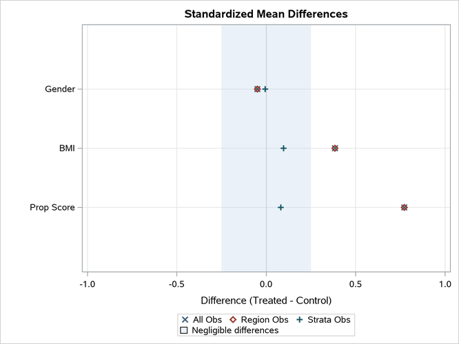
In addition to differences based on all observations and on observations in the support region (which are identical), this plot displays differences based on combining estimates across strata, which are much smaller. For more information about these differences, see the sections Weighting after Stratification and Pooled Standardized Mean Differences across the Strata.
Output 101.2.9 displays a plot of the standardized mean differences for each of the five strata.
Output 101.2.9: Standardized Mean Differences within Strata Plot
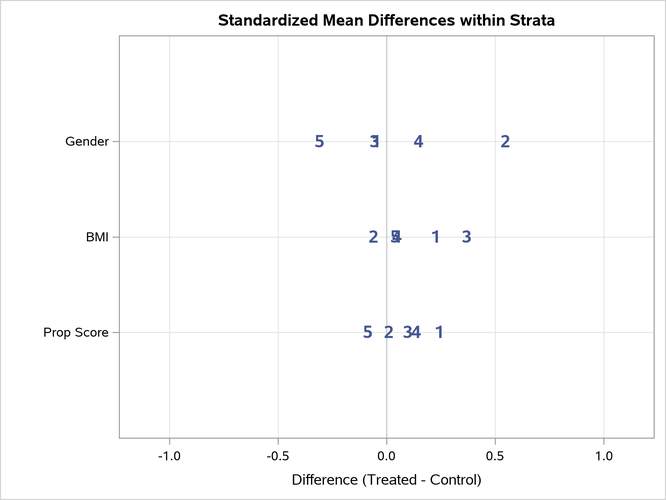
Note that recommended ranges for stratum-specific standardized mean differences are currently not available in the literature.
The "Standardized Mean Differences within Strata" plot corresponds to the "Standardized Mean Differences within Strata" table in Output 101.2.9. The plot reveals larger differences in Stratum 2 and Stratum 5 for Gender.
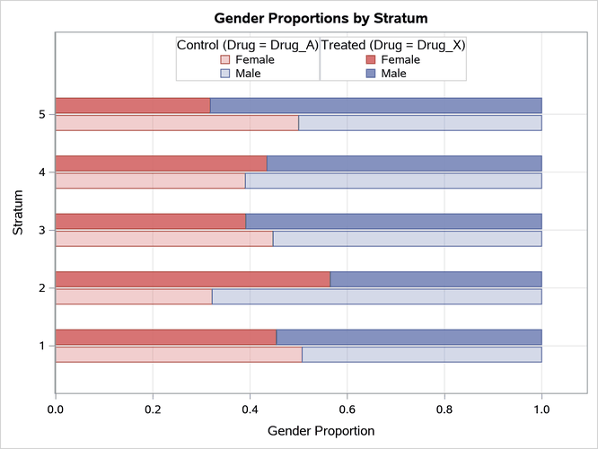
The PLOTS=BARCHART option displays stratum-specific bar charts for the distributions of classification variables in the treated and control groups, as shown in Output 101.2.10 for Gender. Here the largest differences in the distributions occur in Stratum 2 and Stratum 5.
Output 101.2.10: Gender Strata Bar Chart
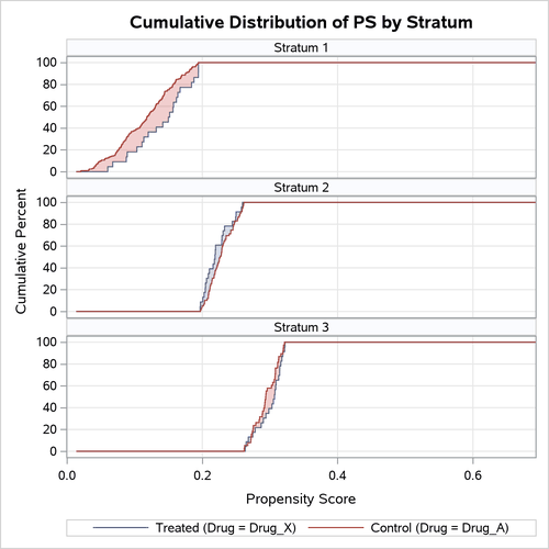
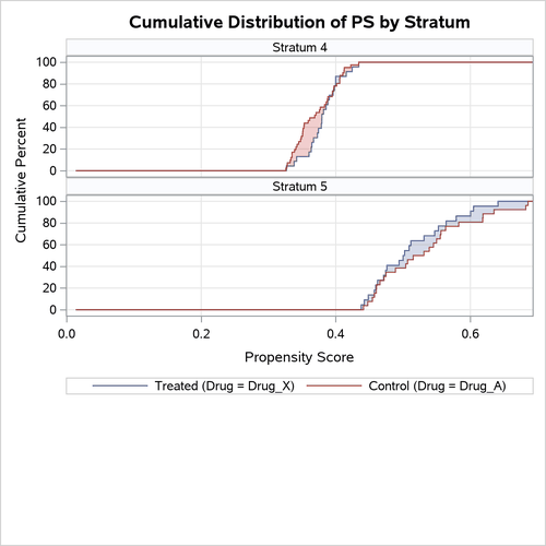
The PLOTS=CDFPLOT option displays stratum-specific CDF plots for the continuous variables in the treated and control groups, as shown in Output 101.2.11 and Output 101.2.12 for PS and in Output 101.2.13 and Output 101.2.14 for BMI.
Output 101.2.11: PS Strata CDF Plot
Output 101.2.12: PS Strata CDF Plot
Output 101.2.13: BMI Strata CDF Plot
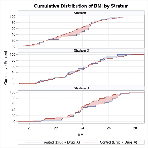
Output 101.2.14: BMI Strata CDF Plot
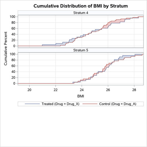
The plots show the differences in the distributions in strata. Here, the largest differences in the distributions of propensity score occur in Stratum 1 (lower values in the control group) and in Stratum 5 (higher values in the treated group)
Because stratification results in good balance for the variables in this example, as shown in Output 101.2.5 and Output 101.2.8, the stratified observations can be saved in an output data set for use in a subsequent outcome analysis.
In situations where you are not satisfied with the variable balance, you can do one or more of the following to improve the balance: you can select another set of variables to fit the propensity score model, you can modify the specification of the propensity score model (for instance, by using nonlinear terms for the continuous variables or by adding interactions), you can increase the number of strata, or you can choose another propensity score method (such as matching).
The OUT(OBS=ALL)=OutEx2 option in the OUTPUT statement creates an output data set named OutEx2 that contains all observations. The following statements list the first 10 observations in OutEx2, which are shown in Output 101.2.15:
proc print data=OutEx2(obs=10);
   var PatientID Drug Gender Age BMI _ps_ _Strata_;
run;
Output 101.2.15: Output Data Set with Strata
| Obs | PatientID | Drug | Gender | Age | BMI | _PS_ | _STRATA_ |
|---|---|---|---|---|---|---|---|
| 1 | 284 | Drug_X | Male | 29 | 22.02 | 0.36444 | 4 |
| 2 | 201 | Drug_A | Male | 45 | 26.68 | 0.22296 | 2 |
| 3 | 147 | Drug_A | Male | 42 | 21.84 | 0.11323 | 1 |
| 4 | 307 | Drug_X | Male | 38 | 22.71 | 0.19733 | 2 |
| 5 | 433 | Drug_A | Male | 31 | 22.76 | 0.35311 | 4 |
| 6 | 435 | Drug_A | Male | 43 | 26.86 | 0.27263 | 3 |
| 7 | 159 | Drug_A | Female | 45 | 25.47 | 0.14911 | 1 |
| 8 | 368 | Drug_A | Female | 49 | 24.28 | 0.07780 | 1 |
| 9 | 286 | Drug_A | Male | 31 | 23.31 | 0.38341 | 4 |
| 10 | 163 | Drug_X | Female | 39 | 25.34 | 0.24995 | 2 |
By default, the output data set includes the variable _PS_, which provides the propensity score, and the variable _STRATA_, which identifies the stratum.
After the responses for the trial are observed, they can be added to the data set OutEx2 as the starting point for an outcome analysis. Assuming that no other confounding variables are associated with both the response variable and the treatment group indicator Drug, you can estimate the treatment effect within each stratum and combine these estimates across strata to estimate the overall treatment effect (Stuart 2010, pp. 13–14). Note that the same stratum weights, as specified in the STRATUMWGT= option in the assessment, should be used in the outcome analysis.