The CAUSALMED Procedure
Causal Mediation Effects: Theory, Definitions, and Effect Decompositions
This section describes the theoretical foundations of the CAUSALMED procedure. It defines the causal mediation and related effects that the procedure estimates, and it describes various types of effect decompositions. The section Causal Mediation Effects: Assumptions, Identification, and Estimation continues the discussion by laying out the assumptions for identifying and estimating causal mediation effects.
In any causal mediation analysis, there are four main types of variables of interest:
an outcome variable Y
a treatment variable T that is hypothesized to have direct and indirect causal effects on the outcome variable Y (in epidemiology, a treatment variable is also known as an exposure, denoted as A)
a mediator variable M that is hypothesized to be causally affected by the treatment variable T and that itself has a direct effect on the outcome variable Y
a set of pretreatment or background covariates that confound the observed relationships among Y, T, and M
Figure 8 represents the first three variables in a causal diagram. A causal diagram depicts the causal relationships of variables in an intuitive way. For a general theory of causal diagrams, see Pearl (2009). The role of the background covariates C is discussed after the causal diagram is interpreted.
Figure 8: A Causal Mediation Model
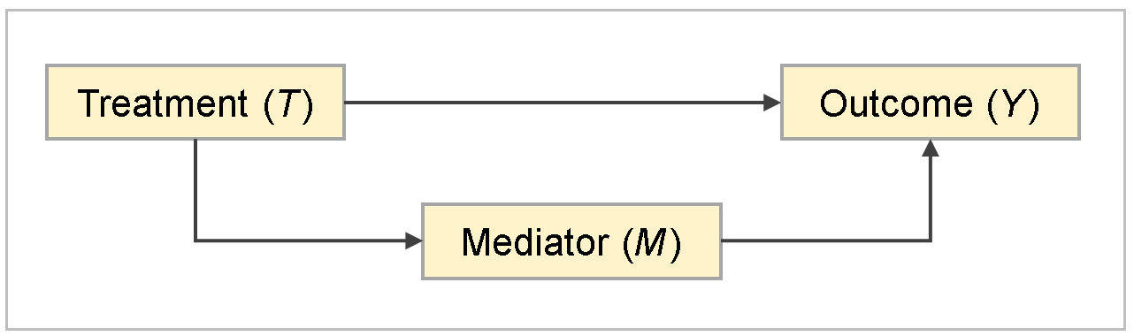
Figure 8 shows two causal pathways that represent the effect of T on Y:
A direct pathway: T
 Y
Y A mediated or indirect pathway: T
M Y
The first causal pathway generates the direct effect of T on Y, and the second pathway generates the indirect effect of T on Y.
Suppose that Y, T, and M are all continuous variables. If you ignore the causal pathways and regress Y on T by using a linear model of the form

where e is an error term that has an expected value of 0 and  is an intercept, then
  is referred to as the total effect of T on Y. This total effect is the overall effect of T on Y without referring to a particular pathway.
When you hypothesize a causal diagram such as Figure 8, the relationships among Y, T, and M are described by two linear equations,

where  and
and  are error terms that have expected values of 0, and the parameters of these two equations are as follows:
 is the intercept of the equation for predicting M.
  is the intercept of the equation for predicting Y.
  is the effect of the T M path.
  is the effect of the T Y path.
  is the effect of the M Y path.
Substituting the equation for predicting M into that for predicting Y, you have

Comparing this equation with the regression equation that predicts Y by T ignoring the causal pathways, you have the equality

where the two terms on the right side of the equation represent additive components of the total effect , assuming that the causal diagram and the corresponding linear equations are true.
Because the first component represents the direct effect of the T Y path, the second component  thus represents the effect of T on Y that is not direct, or simply the indirect effect of T on Y. You can also interpret this indirect effect (
 ) intuitively—it is the product of the two path effects along the indirect pathway T M Y.
Therefore, conceptually, the total effect decomposition can be written as follows:

The direct and indirect effect components are also well defined by the parameters in linear models for continuous Y, T, and M. For an illustration, see Example 38.4.
However, the illustration of the total effect decomposition has been quite ad hoc in nature. It is based on comparing linear models for continuous variables without prior definitions of direct and indirect effects. Consequently, for nonlinear models or linear models that have interaction effects between T and M, the preceding strategy would not work. One reason is that there could be more than two terms in the decomposition so that the direct-indirect decomposition is ambiguous. Another reason is that the terms become much more complicated in nonlinear models, and how to obtain those direct-indirect components would not be clear.
In contrast, the counterfactual framework addresses this issue by offering clear definitions of direct and indirect effects that are applicable to linear and nonlinear models with or without interaction effects. The next section describes this framework.
Another limitation of the illustration that is based solely on the diagram in Figure 8 is that it does not deal adequately with pretreatment characteristics or covariates C in observational studies. Typically, covariates C functions like common causes among Y, T, and M in a causal diagram. In observational studies, the observed associations or relationships among Y, T, and M are attributed to two parts. One part is the actual causal effects among them (that is, the effects that are due to the previously mentioned direct and indirect causal pathways). The other part is their induced associations by C. This part of induced association is often called confounding associations or effects. To obtain unbiased estimates of causal mediation and related effects in observational studies, statistical methods must be able to "remove" the confounding associations. More specifically, the covariates C must suffice to control for confounding of the treatment-outcome, mediator-outcome, and treatment-mediator relationship.
Before a discussion of such statistical methods, a more fundamental issue needs to be addressed: Under what conditions can causal mediation effects be identified? Only after the identification conditions are satisfied can you then attempt to obtain unbiased estimation of causal mediation and related effects. The identification issue is addressed in the section Identification of Causal Mediation Effects after the counterfactual framework is described in the next section. Regression adjustment methods that are based on the identification conditions are then presented in the section Regression Methods for Causal Mediation Analysis.
Counterfactual Framework for Defining Causal Mediation Effects
Mediation analysis has a relatively long history in the field of psychology. Almost all recent developments in the area of causal mediation analysis trace back to the psychological tradition of mediation analysis, as typified by Baron and Kenny (1986). The preceding section illustrates such a traditional approach.
However, as discussed in the preceding section, a problem of the traditional approach is that it lacks a general framework that offers clear definitions of causal mediation and related effects. As a result, the traditional approach cannot deal with interaction effects effectively and it cannot treat binary outcomes and binary mediators in a unified framework.
The counterfactual framework (Robins and Greenland 1992; Pearl 2001) offers a solution to this problem. Within this framework, direct and indirect effects are well defined in terms of counterfactual outcomes. Using these definitions, VanderWeele and Vansteelandt (2009) and VanderWeele and Vansteelandt (2010) derived analytic results for computing causal mediation effects under a wide class of parametric models for various types of treatment and outcome variables. Valeri and VanderWeele (2013) extended these results to binary mediators and count outcomes. VanderWeele (2011) and Valeri and VanderWeele (2015) derived analytic results for analyzing time-to-event (survival) data. This line of development provides the theoretical foundations of the CAUSALMED procedure.
A counterfactual outcome is the outcome that you would observe under a hypothetical intervention that you can set the treatment T to particular level t. Counterfactual outcomes, which are also called potential outcomes by some researchers, are therefore defined for scenarios that might be contrary to the factual outcomes. In the counterfactual framework for causal mediation analysis, interventions on the mediator level are also used in various hypothetical scenarios for defining mediation effects.
The following notation is used for counterfactual outcomes that depend on interventions:
 is the counterfactual outcome of Y for a subject when an intervention sets the treatment level to T = t.
  is the counterfactual outcome of M for a subject when an intervention sets the treatment level to T = t.
  is the counterfactual outcome of Y for a subject when an intervention sets the treatment level to T = t and M = m.
This notation places no restriction on variable types. The variables Y, T, and M can be continuous or binary.
Suppose for the moment that the treatment is binary so that t is either 0 or 1, denoting the control (no treatment) and treatment conditions, respectively. The total effect (TE) for a subject is defined as the difference between the counterfactual outcomes at the treatment and control levels:

In this equation, the first subscript in the counterfactual outcomes denotes the intervention of the treatment (either at 1 or 0), and the second subscript denotes the mediator value that would follow from the intervention of the treatment (either  or
or  ).
).
The controlled direct effect (CDE) for a subject is defined as the difference between the counterfactual outcomes at the two treatment levels when an intervention sets the mediator to a particular level M = m. That is,

The natural direct effect (NDE) for a subject is defined as the difference between the counterfactual outcomes at the two treatment levels when an intervention sets the mediator value to M = , which is the natural level of the mediator when there is no treatment. That is,

The natural indirect effect (NIE) for a subject is defined as the difference between the counterfactual outcomes at the two mediator levels at and when an intervention sets the treatment to T = 1. That is,

All the preceding definitions assume that the treatment variable T is binary. If the treatment variable is continuous, then the treatment levels must be defined according to the treatment and control levels of interest.
For example, if  and
and  are the treatment and control levels on a continuous scale and they represent the levels of substantive interest, they should replace the 1 and 0 values, respectively, for the treatment and control levels in the definitions. However, this more general notation is not used here because it would make the presentation unnecessarily complicated.
These definitions have two important properties. First, they lead to the following conventional two-way decomposition of the total effect (TE):

Second, these definitions are independent of the models for the outcome or mediator. Hence, these definitions and the total effect decomposition are applicable to linear or nonlinear models, with or without an interaction effect between T and M.
The percentage of total effect that is mediated (PM) is computed as

VanderWeele (2014) took a step further and introduces the following four-way decomposition of the total effect:

The component effects in this equation are called the controlled direct effect, the reference interaction, the mediated interaction, and the pure indirect effect, respectively. In VanderWeele (2014), IRF is denoted as  and IMD is denoted as
  . These four component effects are also defined in terms of counterfactual outcomes. For definitions, see VanderWeele (2014).
The significance of these components in causal mediation analysis is that they characterize interaction and mediation effects as follows:
CDE (controlled direct effect) is the component effect that is not due to interaction or mediation.
IRF (reference interaction) is the component effect that is due to interaction but not mediation.
IMD (mediated interaction) is the component effect that is due to both interaction and mediation.
PIE (pure indirect effect) is the component effect that is due to mediation but not interaction.
Dividing each of these component effects by the total effect yields the corresponding proportion contributions of these components. However, these contributions are not interpretable when the components effects have mixed signs.
Some important relationships between the two-way decomposition and the four-way decomposition are expressed by the following equations:

The first equation expresses the natural direct effect (NDE) as the composite component of the controlled direct effect and reference interaction. The second equation expresses the mediation effect or natural indirect effect (NIE) as the composite component of the pure indirect effect and mediated interaction.
Another useful composite component of the four-way decomposition is the "portion attributed to interaction," which is defined as

As its name suggests, this is the portion of the total effect that is due to the interaction between T and M. The percentage of total effect that is due to the interaction is therefore computed as

VanderWeele (2014) discusses various two-way and three-way decompositions and their relationships with the four-way decomposition. He also offers interesting interpretations and applications of these decompositions. For any causal mediation analysis, you can use the DECOMP option in the CAUSALMED procedure to obtain several two-way decompositions, several three-way decompositions, and the four-way decomposition. For more information about the decompositions, see the DECOMP option.
Causal Mediation Estimands
The section Counterfactual Framework for Defining Causal Mediation Effects defines causal mediation and related effects as differences between various counterfactual outcomes for an individual. The presentation is useful for explaining basic concepts. In practice, however, individual causal mediation effects are seldom the target estimands (or population parameters) of interest. This section provides details about the causal mediation estimands. The section Estimands on Difference Scale describes estimands on difference scales, and the section Estimands on Ratio Scale describes estimands on ratio scales.
Estimands on Difference Scale
This section provides details about causal estimands on difference scales. In general, for the regression approach, the total effect estimand can be expressed as the population mean difference between the following two population counterfactual outcomes:

where  is an expectation operation and
  denotes an expectation conditional on the values of covariates C. Let
  be the population mean of C. In all default estimation, PROC CAUSALMED uses
  in place of C to define the causal mediation estimands. That is, the overall total effect estimand on the difference scale is denoted as

It is important to note that this overall total effect is generally not the same as the marginal total effect, which is defined as

However, if the outcome regression model for Y is linear in C, the expectation operator can "pass through" the formula so that the marginal and overall total effects are equivalent.
In summary, for causal mediation effects that are defined on the difference scale, PROC CAUSALMED has the following main default causal estimands:

The total effect decomposition into direct and indirect effects would still have the same additive form as that of the individual total effect decomposition (see the section Counterfactual Framework for Defining Causal Mediation Effects). That is,

Similarly, all formulas for other decompositions that are described in the section Counterfactual Framework for Defining Causal Mediation Effects for individual causal mediation effects apply to the causal estimands that are expressed on the difference scale in this section.
PROC CAUSALMED estimates mean difference causal mediation effects when Y is a continuous outcome that is fitted by a linear model, or when Y is a time-to-event outcome that is fitted by an accelerated failure time model that does not use the log transformation (see the NOLOG option for more information).
In addition to these default mean difference causal mediation estimands, you can estimate similar mean difference effects conditional on particular covariate values for C. For more information about specifying these covariate values and evaluating conditional causal mediation effects, see the EVALUATE statement and the section Evaluating Causal Mediation Effects.
Estimands on Ratio Scale
For Y being fitted by nonlinear outcome models, causal mediation estimands are defined on the ratio scale. This section describes a variety of ratio scale estimands.
For binary outcomes that are fitted by the generalized linear model with a logit link, PROC CAUSALMED has the following main odds ratio estimands:

where is an expectation operation. With the rare outcome assumption (for example, see Valeri and VanderWeele 2013), these odds ratio effect are approximated by their corresponding risk ratio effects. Although these formulas are different from those for defining mean difference mediation effects (see the section Estimands on Difference Scale), both sets of formulas involve the same set of comparisons among counterfactual outcomes conditional on the population mean of C.
For binary outcomes that are fitted by the generalized linear model with the log link, count outcomes that are fitted by the generalized linear model with a Poisson or negative binomial distribution, and time-to-event outcomes that are fitted by the accelerated failure time models, PROC CAUSALMED has the following main risk or mean ratio estimands:

Finally, for time-to-event outcomes that are fitted by the Cox proportional hazards model, PROC CAUSALMED has the following main hazard ratio estimands:

where  denotes the hazard conditional on covariates C at time y.
Again, although mean ratio and hazard ratio effects use different formulas from those for defining mean difference mediation effects (see the section Estimands on Difference Scale), both sets of formulas involve the same set of comparisons among counterfactual outcomes conditional on the population mean of C.
Common to all these ratio scale estimands, the total effect decomposition into direct and indirect effects is not additive, but multiplicative. That is,

The formulas for computing the corresponding percentage mediated, percentage due to interaction, and various decompositions of mean ratio effects are based on the components of the excess of total effect ratio (that is,  ) rather than those of the total effect ratio itself (that is,
  ). Formulas for different cases are quite complicated and therefore are not shown here (but see, for example, VanderWeele 2014).
In addition to these default odds/risk/mean ratio causal mediation estimands, you can estimate similar odds/risk/mean ratio effects conditional on particular covariate values for C. For more information about specifying these covariate values and evaluating conditional causal mediation effects, see the EVALUATE statement and the section Evaluating Causal Mediation Effects.